Creating the boundary forcing#
[1]:
from roms_tools import Grid, BoundaryForcing
As always, the first step is to create our grid. In this example, we choose a grid that contains Greenland’s south east coast and the Irminger Sea. The grid has a horizontal resolution of 2 km and 100 vertical layers.
[2]:
grid = Grid(
    nx=500,
    ny=500,
    size_x=1000,
    size_y=1000,
    center_lon=-37,
    center_lat=63.5,
    rot=25,
    N=100,
    topography_source={
        "name": "SRTM15",
        "path": "/anvil/projects/x-ees250129/Datasets/SRTM15/SRTM15_V2.6.nc",
    },
)
[3]:
grid.plot()
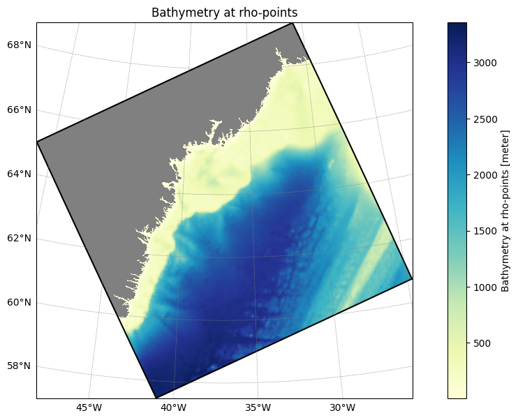
Note that the northern boundary lies entirely on land, so we can exclude it from the boundary forcing generation.
Next, we specify the temporal range that we want to make the surface forcing for.
[3]:
from datetime import datetime
[4]:
start_time = datetime(2012, 1, 30)
end_time = datetime(2012, 2, 4)
ROMS-Tools can create two types of boundary forcing:
physical boundary forcing like temperature, salinity, velocities, and sea surface height
biogeochemical (BGC) boundary forcing like alkalinity, dissolved inorganic phosphate, etc.
As with surface forcing, ROMS accepts multiple boundary forcing files, so we create these two types separately.
Physical boundary forcing#
In this section, we use GLORYS data to create our physical boundary forcing. Our downloaded GLORYS data sits at the following location.
[5]:
glorys_path = [
    "/anvil/projects/x-ees250129/cstar-forge-data/source-data/GLORYS_GLOBAL/cmems_mod_glo_phy_my_0.083deg_P1D-m_GLOBAL_20120129.nc",  # include data from day before start time
    "/anvil/projects/x-ees250129/cstar-forge-data/source-data/GLORYS_GLOBAL/cmems_mod_glo_phy_my_0.083deg_P1D-m_GLOBAL_20120130.nc",
    "/anvil/projects/x-ees250129/cstar-forge-data/source-data/GLORYS_GLOBAL/cmems_mod_glo_phy_my_0.083deg_P1D-m_GLOBAL_20120131.nc",
    "/anvil/projects/x-ees250129/cstar-forge-data/source-data/GLORYS_GLOBAL/cmems_mod_glo_phy_my_0.083deg_P1D-m_GLOBAL_20120201.nc",
    "/anvil/projects/x-ees250129/cstar-forge-data/source-data/GLORYS_GLOBAL/cmems_mod_glo_phy_my_0.083deg_P1D-m_GLOBAL_20120202.nc",
    "/anvil/projects/x-ees250129/cstar-forge-data/source-data/GLORYS_GLOBAL/cmems_mod_glo_phy_my_0.083deg_P1D-m_GLOBAL_20120203.nc",
    "/anvil/projects/x-ees250129/cstar-forge-data/source-data/GLORYS_GLOBAL/cmems_mod_glo_phy_my_0.083deg_P1D-m_GLOBAL_20120204.nc",
    "/anvil/projects/x-ees250129/cstar-forge-data/source-data/GLORYS_GLOBAL/cmems_mod_glo_phy_my_0.083deg_P1D-m_GLOBAL_20120205.nc",  # include data from day after end time
]
Note
We could have also specified the data location via a wildcard, e.g., glorys_path="/anvil/projects/x-ees250129/cstar-forge-data/source-data/GLORYS_GLOBAL/cmems_mod_glo_phy_my_0.083deg_P1D-m_GLOBAL_2012*.nc". But with this latter choice, ROMS-Tools will operate quite a bit slower. More specific filenames are better!
You can also download your own GLORYS data, which must span the desired ROMS domain and temporal range. For more details, please refer to this page.
We now create an instance of the BoundaryForcing class with type = "physics". The boundaries can be provided explicitly as a dictionary, or, if omitted, ROMS-Tools will automatically infer them based on the land/sea mask.
[6]:
%%time

boundary_forcing = BoundaryForcing(
    grid=grid,
    start_time=start_time,
    end_time=end_time,
    boundaries={
        "south": True,
        "east": True,
        "north": False,  # northern boundary excluded
        "west": True,
    },
    source={"name": "GLORYS", "path": glorys_path},
    type="physics",  # "physics" or "bgc"; default is "physics"
    model_reference_date=datetime(2000, 1, 1), # this is the default
    use_dask=True,
)
2026-06-29 18:22:13 - INFO - Using boundary configuration: {'south': True, 'east': True, 'north': False, 'west': True}
CPU times: user 7.39 s, sys: 1.07 s, total: 8.45 s
Wall time: 8.45 s
Note
In the cell above, we created our boundary forcing with use_dask = True. This enables Dask, a Python library designated to facilitate scalable, out-of-memory data processing by distributing computations across multiple threads or processes. Here you can learn more about using Dask with ROMS-Tools.
The boundary forcing variables are held in an xarray.Dataset that is accessible via the .ds property.
[7]:
boundary_forcing.ds
[7]:
<xarray.Dataset> Size: 19MB
Dimensions:     (bry_time: 8, s_rho: 100, xi_u: 501, xi_rho: 502, eta_rho: 502,
                 eta_v: 501)
Coordinates:
    abs_time    (bry_time) datetime64[ns] 64B 2012-01-29 ... 2012-02-05
  * bry_time    (bry_time) float64 64B 4.411e+03 4.412e+03 ... 4.418e+03
Dimensions without coordinates: s_rho, xi_u, xi_rho, eta_rho, eta_v
Data variables: (12/21)
    u_south     (bry_time, s_rho, xi_u) float32 2MB dask.array<chunksize=(1, 100, 501), meta=np.ndarray>
    v_south     (bry_time, s_rho, xi_rho) float32 2MB dask.array<chunksize=(1, 100, 502), meta=np.ndarray>
    temp_south  (bry_time, s_rho, xi_rho) float32 2MB dask.array<chunksize=(1, 100, 502), meta=np.ndarray>
    salt_south  (bry_time, s_rho, xi_rho) float32 2MB dask.array<chunksize=(1, 100, 502), meta=np.ndarray>
    zeta_south  (bry_time, xi_rho) float32 16kB dask.array<chunksize=(1, 502), meta=np.ndarray>
    ubar_south  (bry_time, xi_u) float32 16kB dask.array<chunksize=(1, 501), meta=np.ndarray>
    ...          ...
    v_west      (bry_time, s_rho, eta_v) float32 2MB dask.array<chunksize=(1, 100, 501), meta=np.ndarray>
    temp_west   (bry_time, s_rho, eta_rho) float32 2MB dask.array<chunksize=(1, 100, 502), meta=np.ndarray>
    salt_west   (bry_time, s_rho, eta_rho) float32 2MB dask.array<chunksize=(1, 100, 502), meta=np.ndarray>
    zeta_west   (bry_time, eta_rho) float32 16kB dask.array<chunksize=(1, 502), meta=np.ndarray>
    ubar_west   (bry_time, eta_rho) float32 16kB dask.array<chunksize=(1, 502), meta=np.ndarray>
    vbar_west   (bry_time, eta_v) float32 16kB dask.array<chunksize=(1, 501), meta=np.ndarray>
Attributes: (12/13)
    title:                                ROMS boundary forcing file created ...
    roms_tools_version:                   10000.dev377+g7f6dd1f62
    start_time:                           2012-01-30 00:00:00
    end_time:                             2012-02-04 00:00:00
    source:                               GLORYS
    model_reference_date:                 2000-01-01 00:00:00
    ...                                   ...
    regrid_method:                        xesmf
    extrap_method:                        inverse_dist
    adjust_depth_for_sea_surface_height:  False
    theta_s:                              5.0
    theta_b:                              2.0
hc: 300.0All physical boundary forcing fields necessary to run a ROMS simulation are now contained as dask.arrays within an xarray.Dataset. All data operations are performed lazily, meaning that the surface forcing fields have not been actually computed yet. Full computation will not be triggered until the .save method is called.
[8]:
boundary_forcing.ds.bry_time
[8]:
<xarray.DataArray 'bry_time' (bry_time: 8)> Size: 64B
array([4411., 4412., 4413., 4414., 4415., 4416., 4417., 4418.])
Coordinates:
    abs_time  (bry_time) datetime64[ns] 64B 2012-01-29 2012-01-30 ... 2012-02-05
  * bry_time  (bry_time) float64 64B 4.411e+03 4.412e+03 ... 4.417e+03 4.418e+03
Attributes:
    long_name:  relative time: days since 2000-01-01 00:00:00
units: daysNote
The bry_time variable shows relative time, i.e., days since the model reference date (here set to January 1, 2000 by default). The abs_time coordinate shows the absolute time. The GLORYS data provided to ROMS-Tools has daily frequency; this temporal frequency is inherited by boundary_forcing.
boundary_forcing has 8 time entries because ROMS-Tools makes sure to include one time entry at or before the start_time, and one time entry at or after the end_time. This is essential for proper functioning within ROMS. If the provided data does not meet this requirement, ROMS-Tools will issue a warning.
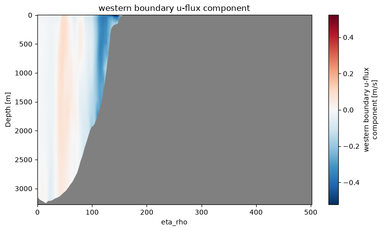
Let’s make some plots! As an example, let’s have a look at the zonal velocity field u at the southern and western boundaries.
[9]:
boundary_forcing.plot("u_south", time=0, layer_contours=True)
[########################################] | 100% Completed | 202.56 ms
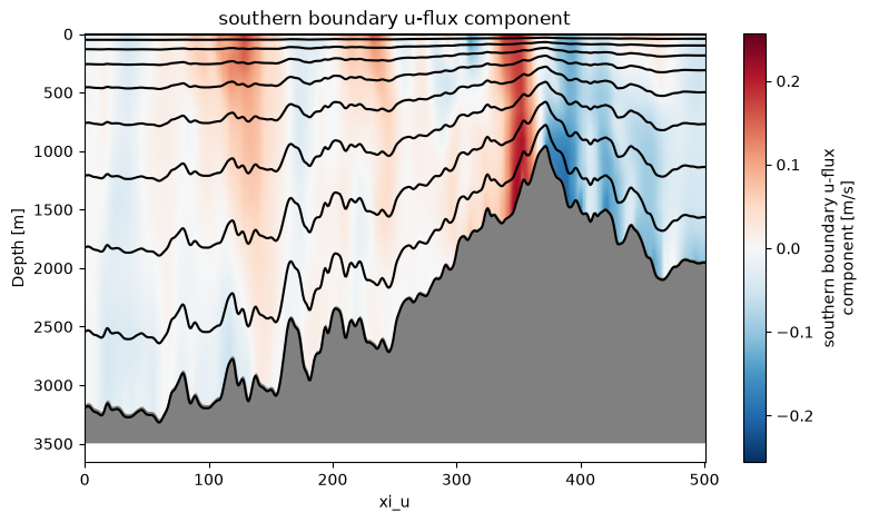
Note that even though we have a total of 100 layers, layer_contours = True will create a plot with a maximum of 10 contours to ensure plot clarity.
[10]:
boundary_forcing.plot("u_west", time=0, layer_contours=False)
[########################################] | 100% Completed | 202.82 ms
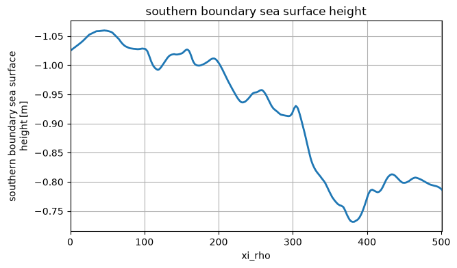
Sea surface height zeta at any of the boundaries and for a specific time is only a 1D variable.
[11]:
boundary_forcing.plot("zeta_south", time=0)
[########################################] | 100% Completed | 101.41 ms
The same is true for the barotropic velocity ubar.
[12]:
boundary_forcing.plot("ubar_east", time=0)
[########################################] | 100% Completed | 202.86 ms

Biogeochemical (BGC) boundary forcing#
We now create BGC boundary forcing. The BGC variables are interpolated from a climatology with 1° horizontal resolution, using the following approach:
The BGC climatology can be accessed at the following location:
[13]:
unified_bgc_path = "/anvil/projects/x-ees250129/Datasets/UNIFIED/BGCdataset.nc"
[16]:
%%time

unified_bgc_boundary_forcing = BoundaryForcing(
    grid=grid,
    start_time=start_time,
    end_time=end_time,
    source={"name": "UNIFIED", "path": unified_bgc_path, "climatology": True},
    type="bgc",
    use_dask=True,
)
2026-06-29 18:22:25 - INFO - No `boundaries` provided. Using mask-based defaults: {'south': True, 'east': True, 'north': False, 'west': True}
2026-06-29 18:22:25 - WARNING - Optional variables missing (but not critical): ['Lig', 'DIC_ALT_CO2', 'Alk_ALT_CO2', 'temp_WOA', 'salt_WOA']
CPU times: user 1.37 s, sys: 32.8 ms, total: 1.4 s
Wall time: 1.41 s
[17]:
unified_bgc_boundary_forcing.ds
[17]:
<xarray.Dataset> Size: 231MB
Dimensions:            (bry_time: 12, s_rho: 100, xi_rho: 502, eta_rho: 502)
Coordinates:
    month              (bry_time) int64 96B 1 2 3 4 5 6 7 8 9 10 11 12
    abs_time           (bry_time) datetime64[ns] 96B 2000-01-16T12:00:00 ... ...
  * bry_time           (bry_time) float64 96B 15.5 45.0 74.5 ... 319.0 349.5
Dimensions without coordinates: s_rho, xi_rho, eta_rho
Data variables: (12/96)
    PO4_south          (bry_time, s_rho, xi_rho) float32 2MB dask.array<chunksize=(1, 100, 502), meta=np.ndarray>
    NO3_south          (bry_time, s_rho, xi_rho) float32 2MB dask.array<chunksize=(1, 100, 502), meta=np.ndarray>
    SiO3_south         (bry_time, s_rho, xi_rho) float32 2MB dask.array<chunksize=(1, 100, 502), meta=np.ndarray>
    Fe_south           (bry_time, s_rho, xi_rho) float32 2MB dask.array<chunksize=(1, 100, 502), meta=np.ndarray>
    O2_south           (bry_time, s_rho, xi_rho) float32 2MB dask.array<chunksize=(1, 100, 502), meta=np.ndarray>
    DIC_south          (bry_time, s_rho, xi_rho) float32 2MB dask.array<chunksize=(1, 100, 502), meta=np.ndarray>
    ...                 ...
    diazFe_west        (bry_time, s_rho, eta_rho) float32 2MB dask.array<chunksize=(1, 100, 502), meta=np.ndarray>
    spCaCO3_west       (bry_time, s_rho, eta_rho) float32 2MB dask.array<chunksize=(1, 100, 502), meta=np.ndarray>
    zooC_west          (bry_time, s_rho, eta_rho) float32 2MB dask.array<chunksize=(1, 100, 502), meta=np.ndarray>
    Lig_west           (bry_time, s_rho, eta_rho) float32 2MB dask.array<chunksize=(1, 100, 502), meta=np.ndarray>
    DIC_ALT_CO2_west   (bry_time, s_rho, eta_rho) float32 2MB dask.array<chunksize=(1, 100, 502), meta=np.ndarray>
    ALK_ALT_CO2_west   (bry_time, s_rho, eta_rho) float32 2MB dask.array<chunksize=(1, 100, 502), meta=np.ndarray>
Attributes: (12/14)
    title:                                ROMS boundary forcing file created ...
    roms_tools_version:                   10000.dev377+g7f6dd1f62
    start_time:                           2012-01-30 00:00:00
    end_time:                             2012-02-04 00:00:00
    source:                               UNIFIED
    model_reference_date:                 2000-01-01 00:00:00
    ...                                   ...
    extrap_method:                        inverse_dist
    adjust_depth_for_sea_surface_height:  False
    theta_s:                              5.0
    theta_b:                              2.0
    hc:                                   300.0
climatology: TrueLet’s investigate the time variable of our dataset.
[19]:
unified_bgc_boundary_forcing.ds["bry_time"]
[19]:
<xarray.DataArray 'bry_time' (bry_time: 12)> Size: 96B
array([ 15.5,  45. ,  74.5, 105. , 135.5, 166. , 196. , 227.5, 258. , 288.5,
       319. , 349.5])
Coordinates:
month (bry_time) int64 96B 1 2 3 4 5 6 7 8 9 10 11 12
abs_time (bry_time) datetime64[ns] 96B 2000-01-16T12:00:00 ... 2000-12-1...
* bry_time (bry_time) float64 96B 15.5 45.0 74.5 105.0 ... 288.5 319.0 349.5
Attributes:
cycle_length: 365.25
long_name: relative time: days since 2000-01-01 00:00:00
units: daysNote
The dataset unified_bgc_boundary_forcing.ds contains twelve time entries because its respective source is a climatology, as we specified via source["climatology"] = True.
For climatologies, ROMS-Tools does not subsample the twelve time entries further, regardless of the provided start and end time. Note that the bry_time coordinate has an additional attribute: cycle_length (with units in days). This attribute will tell ROMS to repeat the climatology every 365.25 days. In other words, the data in bgc_boundary_forcing.ds will work for ROMS run over any time window (as long as the model reference date is January 1, xxxx).
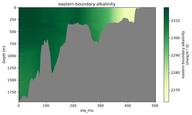
We can plot the BGC boundary forcing as we saw above.
[21]:
unified_bgc_boundary_forcing.plot("ALK_east", time=0)
[########################################] | 100% Completed | 101.31 ms
Interpolate BGC variables by density or mixed-layer depth instead of plain depth#
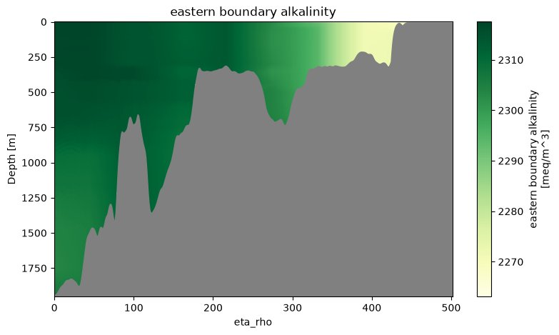
By default (bgc_interpolation_method="depth"), BGC tracers are interpolated onto the model’s vertical grid in depth. Because biogeochemical fields tend to follow water masses rather than fixed depths, two alternatives are available:
bgc_interpolation_method="density"interpolates the tracers in potential-density (isopycnal) space. The density coordinate is built from the BGC dataset’s own temperature/salinity for the source profile and from the model’s temperature/salinity for the target.bgc_interpolation_method="density_mld"finds the mixed layer depth (MLD) in the source and target density fields, scales the source mixed layer so its MLD matches the target’s, and then interpolates 1:1 in depth below the MLD. This keeps the mixed layers aligned and preserves the absolute depth of sub-mixed-layer features, while avoiding the surface degeneracy of pure density space.
For boundary forcing, the density methods also need the physics boundary forcing object, passed as e.g. physics_forcing=boundary_forcing.
Both density methods require the BGC source to provide temperature/salinity (e.g. the unified dataset’s temp_WOA/salt_WOA); otherwise interpolation falls back to depth space.
[22]:
%%time

unified_bgc_boundary_forcing_mld = BoundaryForcing(
    grid=grid,
    start_time=start_time,
    end_time=end_time,
    source={"name": "UNIFIED", "path": unified_bgc_path, "climatology": True},
    type="bgc",
    use_dask=True,
    bgc_interpolation_method="density_mld",
    physics_forcing=boundary_forcing,  # physics T/S supplies the target density
)
2026-06-29 18:22:27 - INFO - No `boundaries` provided. Using mask-based defaults: {'south': True, 'east': True, 'north': False, 'west': True}
2026-06-29 18:22:27 - WARNING - Optional variables missing (but not critical): ['Lig', 'DIC_ALT_CO2', 'Alk_ALT_CO2', 'temp_WOA', 'salt_WOA']
2026-06-29 18:22:28 - INFO - 'density_mld' interpolation requested but the BGC source has no temperature/salinity; falling back to depth-space interpolation (south boundary).
2026-06-29 18:22:28 - INFO - 'density_mld' interpolation requested but the BGC source has no temperature/salinity; falling back to depth-space interpolation (east boundary).
2026-06-29 18:22:29 - INFO - 'density_mld' interpolation requested but the BGC source has no temperature/salinity; falling back to depth-space interpolation (west boundary).
CPU times: user 1.85 s, sys: 28.8 ms, total: 1.88 s
Wall time: 1.88 s
[23]:
unified_bgc_boundary_forcing_mld.plot("ALK_east", time=0)
[########################################] | 100% Completed | 101.25 ms
Saving as NetCDF or YAML file#
We can now save our boundary forcings as a NetCDF files.
We need to specify the desired target path.
[24]:
filepath = "/anvil/scratch/x-kthyng/forcing/my_bgc_boundary_forcing.nc"
[25]:
%time unified_bgc_boundary_forcing.save(filepath)
2026-06-29 18:22:44 - INFO - Writing the following NetCDF files:
/anvil/scratch/x-kthyng/forcing/my_bgc_boundary_forcing_clim.nc
[########################################] | 100% Completed | 7.36 ss
CPU times: user 6.94 s, sys: 2.39 s, total: 9.32 s
Wall time: 8.05 s
[25]:
[PosixPath('/anvil/scratch/x-kthyng/forcing/my_bgc_boundary_forcing_clim.nc')]
Next, let’s save the physical boundary forcing. We will use the group = True flag (default) which ensures that the data is split into multiple NetCDFs, grouped into months.
[26]:
filepath = "/anvil/scratch/x-kthyng/forcing/my_boundary_forcing.nc"
[27]:
%time boundary_forcing.save(filepath, group=True)
2026-06-29 18:22:52 - INFO - Writing the following NetCDF files:
/anvil/scratch/x-kthyng/forcing/my_boundary_forcing_201201.nc
/anvil/scratch/x-kthyng/forcing/my_boundary_forcing_201202.nc
[########################################] | 100% Completed | 7.06 ss
[########################################] | 100% Completed | 19.01 s
CPU times: user 3.79 s, sys: 4.21 s, total: 8 s
Wall time: 27.4 s
[27]:
[PosixPath('/anvil/scratch/x-kthyng/forcing/my_boundary_forcing_201201.nc'),
 PosixPath('/anvil/scratch/x-kthyng/forcing/my_boundary_forcing_201202.nc')]
From the file paths printed to the screen, you will notice that the year and month information has been appended to the specified path.
Note
The way data is grouped depends on its temporal frequency. For datasets with a daily or higher frequency, the data is grouped by month. For datasets with lower temporal frequency (e.g., monthly data), the grouping is done by year.
We can also export the parameters of our BoundaryForcing object to a YAML file.
[31]:
yaml_filepath = "/anvil/scratch/x-kthyng/forcing/my_boundary_forcing.yaml"
[32]:
boundary_forcing.to_yaml(yaml_filepath)
This is the YAML file that was created.
[33]:
# Open and read the YAML file
with open(yaml_filepath, "r") as file:
    file_contents = file.read()

# Print the contents
print(file_contents)
---
roms_tools_version: 10000.dev377+g7f6dd1f62
---
Grid:
  nx: 500
  ny: 500
  size_x: 1000
  size_y: 1000
  center_lon: -37
  center_lat: 63.5
  rot: 25
  N: 100
  theta_s: 5.0
  theta_b: 2.0
  hc: 300.0
  topography_source:
    name: SRTM15
    path: /anvil/projects/x-ees250129/Datasets/SRTM15/SRTM15_V2.6.nc
  mask_shapefile: null
  close_narrow_channels: false
  hmin: 5.0
  filename: null
BoundaryForcing:
  start_time: '2012-01-30T00:00:00'
  end_time: '2012-02-04T00:00:00'
  boundaries:
    south: true
    east: true
    north: false
    west: true
  source:
    name: GLORYS
    path:
    - /anvil/projects/x-ees250129/cstar-forge-data/source-data/GLORYS_GLOBAL/cmems_mod_glo_phy_my_0.083deg_P1D-m_GLOBAL_20120129.nc
    - /anvil/projects/x-ees250129/cstar-forge-data/source-data/GLORYS_GLOBAL/cmems_mod_glo_phy_my_0.083deg_P1D-m_GLOBAL_20120130.nc
    - /anvil/projects/x-ees250129/cstar-forge-data/source-data/GLORYS_GLOBAL/cmems_mod_glo_phy_my_0.083deg_P1D-m_GLOBAL_20120131.nc
    - /anvil/projects/x-ees250129/cstar-forge-data/source-data/GLORYS_GLOBAL/cmems_mod_glo_phy_my_0.083deg_P1D-m_GLOBAL_20120201.nc
    - /anvil/projects/x-ees250129/cstar-forge-data/source-data/GLORYS_GLOBAL/cmems_mod_glo_phy_my_0.083deg_P1D-m_GLOBAL_20120202.nc
    - /anvil/projects/x-ees250129/cstar-forge-data/source-data/GLORYS_GLOBAL/cmems_mod_glo_phy_my_0.083deg_P1D-m_GLOBAL_20120203.nc
    - /anvil/projects/x-ees250129/cstar-forge-data/source-data/GLORYS_GLOBAL/cmems_mod_glo_phy_my_0.083deg_P1D-m_GLOBAL_20120204.nc
    - /anvil/projects/x-ees250129/cstar-forge-data/source-data/GLORYS_GLOBAL/cmems_mod_glo_phy_my_0.083deg_P1D-m_GLOBAL_20120205.nc
    climatology: false
  type: physics
  prefill: null
  prefill_kwargs: null
  regrid_method: null
  extrap_method: null
  extrap_kwargs: null
  model_reference_date: '2000-01-01T00:00:00'
  chunks: null
  initial_slice_bounds: null
  bypass_validation: false
  bgc_interpolation_method: depth
Creating boundary forcing from an existing YAML file#
[34]:
%time the_same_boundary_forcing = BoundaryForcing.from_yaml(yaml_filepath, use_dask=True)
2026-06-29 18:25:44 - INFO - Using boundary configuration: {'south': True, 'east': True, 'north': False, 'west': True}
CPU times: user 9.74 s, sys: 1.15 s, total: 10.9 s
Wall time: 12.8 s
[35]:
the_same_boundary_forcing.ds
[35]:
<xarray.Dataset> Size: 19MB
Dimensions:     (bry_time: 8, s_rho: 100, xi_u: 501, xi_rho: 502, eta_rho: 502,
                 eta_v: 501)
Coordinates:
    abs_time    (bry_time) datetime64[ns] 64B 2012-01-29 ... 2012-02-05
  * bry_time    (bry_time) float64 64B 4.411e+03 4.412e+03 ... 4.418e+03
Dimensions without coordinates: s_rho, xi_u, xi_rho, eta_rho, eta_v
Data variables: (12/21)
    u_south     (bry_time, s_rho, xi_u) float32 2MB dask.array<chunksize=(1, 100, 501), meta=np.ndarray>
    v_south     (bry_time, s_rho, xi_rho) float32 2MB dask.array<chunksize=(1, 100, 502), meta=np.ndarray>
    temp_south  (bry_time, s_rho, xi_rho) float32 2MB dask.array<chunksize=(1, 100, 502), meta=np.ndarray>
    salt_south  (bry_time, s_rho, xi_rho) float32 2MB dask.array<chunksize=(1, 100, 502), meta=np.ndarray>
    zeta_south  (bry_time, xi_rho) float32 16kB dask.array<chunksize=(1, 502), meta=np.ndarray>
    ubar_south  (bry_time, xi_u) float32 16kB dask.array<chunksize=(1, 501), meta=np.ndarray>
    ...          ...
    v_west      (bry_time, s_rho, eta_v) float32 2MB dask.array<chunksize=(1, 100, 501), meta=np.ndarray>
    temp_west   (bry_time, s_rho, eta_rho) float32 2MB dask.array<chunksize=(1, 100, 502), meta=np.ndarray>
    salt_west   (bry_time, s_rho, eta_rho) float32 2MB dask.array<chunksize=(1, 100, 502), meta=np.ndarray>
    zeta_west   (bry_time, eta_rho) float32 16kB dask.array<chunksize=(1, 502), meta=np.ndarray>
    ubar_west   (bry_time, eta_rho) float32 16kB dask.array<chunksize=(1, 502), meta=np.ndarray>
    vbar_west   (bry_time, eta_v) float32 16kB dask.array<chunksize=(1, 501), meta=np.ndarray>
Attributes: (12/13)
    title:                                ROMS boundary forcing file created ...
    roms_tools_version:                   10000.dev377+g7f6dd1f62
    start_time:                           2012-01-30 00:00:00
    end_time:                             2012-02-04 00:00:00
    source:                               GLORYS
    model_reference_date:                 2000-01-01 00:00:00
    ...                                   ...
    regrid_method:                        xesmf
    extrap_method:                        inverse_dist
    adjust_depth_for_sea_surface_height:  False
    theta_s:                              5.0
    theta_b:                              2.0
hc: 300.0Horizontal regridding near land and coarse source data#
The source data (such as GLORYS) and the ROMS grid generally have different land masks, often because they have different resolutions. A naive linear interpolation would propagate NaNs into the ROMS boundary wherever any of the surrounding source cells is land, leaving holes at ocean points that ROMS needs.
ROMS-Tools avoids this with a NaN-aware horizontal regridding that needs no separate fill step:
When xESMF is available (the default for conda installs), boundary data is regridded with masked bilinear interpolation: the interpolation weights are renormalized over only the valid (ocean) source cells, so a target point surrounded by mostly land still receives a sensible ocean value. Target points whose source neighbors are all land are then filled by inverse-distance-weighted extrapolation (configurable via the
extrap_methodargument). Together these guarantee NaN-free boundaries.When xESMF is not available (e.g. Windows/pip installs),
ROMS-Toolsfalls back to a nearest-neighbor pre-fill of the source data followed by scipy linear interpolation. Because every masked source cell is first filled with its nearest valid ocean value, the subsequent interpolation cannot propagate NaNs. This is numerically close to, though not identical to, the masked-bilinear result.
This replaces the older, slower 2D Poisson (AMG) fill that was previously required to plug NaN holes before regridding, giving a substantial speedup and memory reduction on large, multi-year domains.
You can also choose the regrid engine explicitly with the regrid_method argument ("auto" (default; xESMF if installed, otherwise scipy), "xesmf", or "scipy"), independently of any source pre-fill, and tune the extrapolation with extrap_kwargs (e.g. num_src_pnts and dist_exponent for "inverse_dist").
Coarse resolution of the source data#
Now let’s look at the second difficult case: source data that is so coarse that a ROMS boundary may appear to lie almost entirely on land in the source grid. We create a grid around the waters surrounding Wales.
[36]:
grid = Grid(
    nx=30,
    ny=30,
    size_x=240,
    size_y=240,
    center_lon=-4.1,
    center_lat=52.36,
    rot=0,
    topography_source={
        "name": "SRTM15",
        "path": "/anvil/projects/x-ees250129/Datasets/SRTM15/SRTM15_V2.6.nc",
    },
)
[43]:
grid.plot()
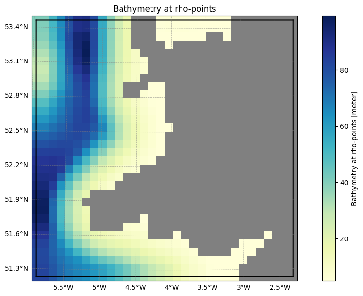
Before generating the boundary forcing, let’s first examine the source data that we will be regridding. For this example, we use BGC data from a coarse 1x1 degree CESM simulation. The use of CESM is simply for demonstration purposes, but this same method can be applied to GLORYS.
[37]:
import xarray as xr
[ ]:
cesm_bgc_path = "/anvil/projects/x-ees250129/Datasets/CESM_REGRIDDED/CESM-climatology_lowres_regridded.nc"
[38]:
ds_source = xr.open_dataset(cesm_bgc_path)
ds_source
[38]:
<xarray.Dataset> Size: 4GB
Dimensions:      (month: 12, z_t: 60, lat: 180, lon: 360, z_t_150m: 15)
Coordinates:
  * month        (month) int64 96B 1 2 3 4 5 6 7 8 9 10 11 12
  * z_t          (z_t) float32 240B 500.0 1.5e+03 ... 5.125e+05 5.375e+05
  * z_t_150m     (z_t_150m) float32 60B 500.0 1.5e+03 ... 1.35e+04 1.45e+04
  * lon          (lon) float64 3kB -179.5 -178.5 -177.5 ... 177.5 178.5 179.5
  * lat          (lat) float64 1kB -89.5 -88.5 -87.5 -86.5 ... 87.5 88.5 89.5
Data variables: (12/32)
    ALK          (month, z_t, lat, lon) float32 187MB ...
    ALK_ALT_CO2  (month, z_t, lat, lon) float32 187MB ...
    DIC          (month, z_t, lat, lon) float32 187MB ...
    DIC_ALT_CO2  (month, z_t, lat, lon) float32 187MB ...
    DOC          (month, z_t, lat, lon) float32 187MB ...
    DOCr         (month, z_t, lat, lon) float32 187MB ...
    ...           ...
    spC          (month, z_t_150m, lat, lon) float32 47MB ...
    spCaCO3      (month, z_t_150m, lat, lon) float32 47MB ...
    spChl        (month, z_t_150m, lat, lon) float32 47MB ...
    spFe         (month, z_t_150m, lat, lon) float32 47MB ...
    spP          (month, z_t_150m, lat, lon) float32 47MB ...
    zooC         (month, z_t_150m, lat, lon) float32 47MB ...
Attributes:
    Title:          Climatology computed from the 1x1 degree CESM-MARBL simul...
    original_path:  /glade/campaign/collections/cmip/CMIP6/CESM-HR/FOSI_BGC/L...
regrid_method: conservativeHere, we zoom in on the coarse CESM source data around the Wales domain of interest.
[40]:
import matplotlib.pyplot as plt

fig, ax = plt.subplots()
ds_source["ALK"].isel(z_t=0, month=0).sel(lat=slice(40, 60), lon=slice(-20, 0)).plot(
    ax=ax
)
lon_min = grid.ds.lon_rho.min() - 360
lon_max = grid.ds.lon_rho.max() - 360
lat_min = grid.ds.lat_rho.min()
lat_max = grid.ds.lat_rho.max()

ax.plot(
    [lon_min, lon_min, lon_max, lon_max, lon_min],
    [lat_min, lat_max, lat_max, lat_min, lat_min],
    color="r",
    linewidth=2,
    label="ROMS domain",
)
ax.legend(loc="upper left")
[40]:
<matplotlib.legend.Legend at 0x1474748c2900>
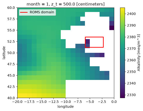
As shown above, all the boundaries of this ROMS domain lie almost entirely on land in the coarse 1x1 degree CESM source, with at most one ocean grid point per boundary. Previously, skipping the 2D fill in this situation produced boundaries that were entirely NaN, and ROMS-Tools raised an error.
With the NaN-aware default this is no longer a problem: masked bilinear interpolation uses the few available ocean source cells, and inverse-distance extrapolation fills any boundary points whose source neighbors are all land. Every boundary point therefore receives a finite value without any 2D fill. In such extreme cases (a source much coarser than the grid) the boundary values should be inspected, since the extrapolation is connectivity-blind and could pull a value from the wrong side of a narrow land barrier.
Pre-filling the source data#
The default NaN-aware regridding above interpolates directly from the valid ocean cells of the source. In some cases you may instead want to fill the source’s land/void cells first and then regrid the now NaN-free source. This is controlled by the prefill argument (with method-specific options in prefill_kwargs):
Strategy |
|
Needs xESMF |
Cost |
Character |
|---|---|---|---|---|
Masked bilinear + extrapolation (default) |
|
yes* |
low |
Interpolates over real ocean only; |
AMG Poisson fill (legacy) |
|
no |
high |
Smoothest; a global harmonic fill of the whole source. Slower and more memory-hungry on large domains. |
Inverse-distance fill |
|
yes |
medium |
Smooth inverse-distance-weighted fill of the source; tune with |
Nearest-source fill |
|
yes |
low |
Blocky (single nearest source cell). |
Nearest-neighbor fill |
|
no |
lowest |
Blocky and connectivity-blind; also the automatic fallback when xESMF is unavailable. |
There are two independent stages here: ``prefill`` fills the source before regridding (after which the regrid is a plain bilinear interpolation, so extrap_method no longer applies), while ``extrap_method`` fills destination boundary points during the default masked-bilinear regrid. The regrid engine itself is selected with regrid_method ("auto", "xesmf", "scipy").
Let’s visualize how each method fills the coarse CESM source over the Wales domain. We crop the source to the domain (plus a buffer) and apply each fill in turn:
[42]:
from roms_tools.datasets.lat_lon_datasets import CESMBGCDataset
from roms_tools.setup.utils import get_target_coords

target_coords = get_target_coords(grid)
source = CESMBGCDataset(
    filename=cesm_bgc_path,
    start_time=start_time,
    end_time=end_time,
    climatology=True,
    use_dask=True,
)

lon_name = source.dim_names["longitude"]
lat_name = source.dim_names["latitude"]

methods = ["2d_lateral_fill", "inverse_dist", "nearest_s2d", "nearest_neighbor"]
fig, axs = plt.subplots(2, 2, figsize=(11, 9), constrained_layout=True)

for method, ax in zip(methods, axs.ravel()):
    # A fresh copy per method so each fill starts from the raw (NaN) source.
    sub = source.choose_subdomain(
        target_coords, return_copy=True, unchunk_lateral_dims=True
    )
    sub.convert_to_float64()
    sub.extrapolate_deepest_to_bottom()   # fill deep NaNs down each column first
    sub.apply_prefill(method)

    field = sub.ds["ALK"]
    # reduce to a single (lat, lon) surface slice for plotting
    extra_dims = [d for d in field.dims if d not in (lon_name, lat_name)]
    field.isel({d: 0 for d in extra_dims}).plot(ax=ax, x=lon_name, y=lat_name)
    ax.set_title(f"prefill='{method}'")
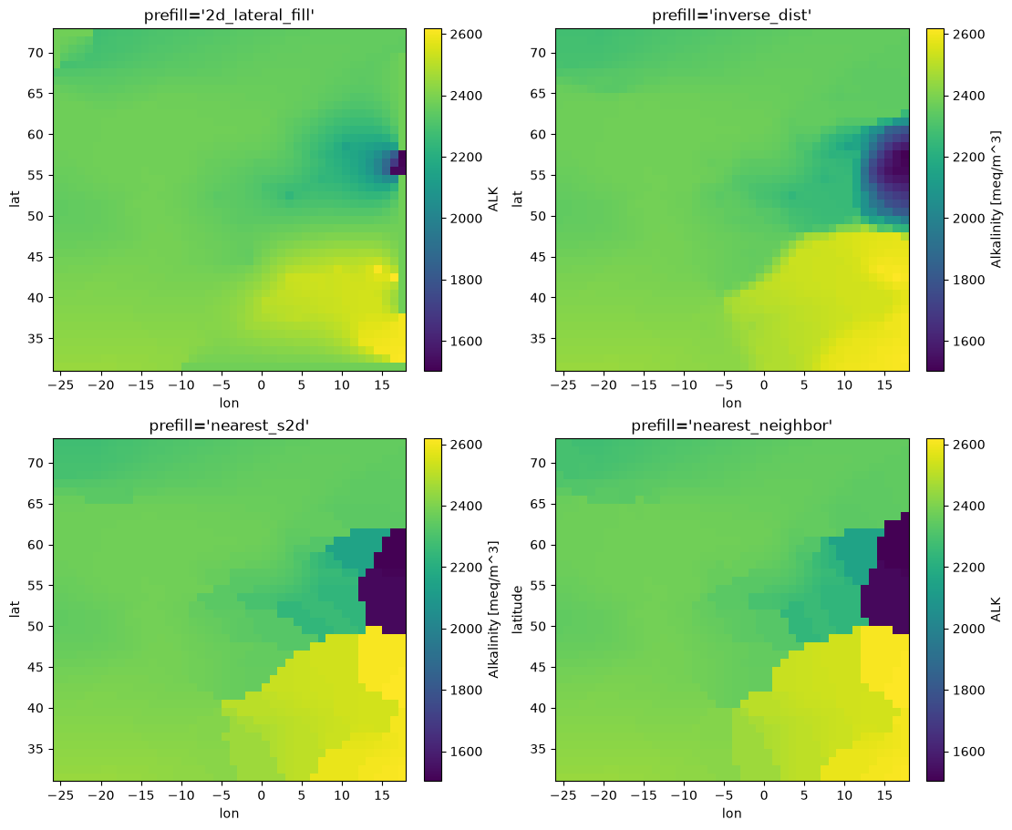
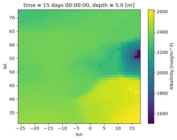
The AMG (2d_lateral_fill) and inverse-distance fills produce smooth fields, while the two nearest-style fills are blockier. For inverse_dist you can trade smoothness against locality via prefill_kwargs (more source points and a smaller distance exponent give a smoother fill):
[43]:
sub = source.choose_subdomain(
    target_coords, return_copy=True, unchunk_lateral_dims=True
)
sub.convert_to_float64()
sub.apply_prefill(
    "inverse_dist", prefill_kwargs={"num_src_pnts": 16, "dist_exponent": 1.0}
)

field = sub.ds["ALK"]
extra_dims = [d for d in field.dims if d not in (lon_name, lat_name)]
field.isel({d: 0 for d in extra_dims}).plot(x=lon_name, y=lat_name)
[43]:
<matplotlib.collections.QuadMesh at 0x14717f99c910>
To use a pre-fill when building the physics boundary forcing itself, pass prefill (and optionally prefill_kwargs and regrid_method) to BoundaryForcing:
bf = BoundaryForcing(
    grid=grid,
    start_time=start_time,
    end_time=end_time,
    boundaries={
        "south": True,
        "east": True,
        "north": False,  # northern boundary excluded
        "west": True,
    },
    source={"name": "GLORYS", "path": glorys_path},
    type="physics",  # "physics" or "bgc"; default is "physics"
    prefill="inverse_dist",
    prefill_kwargs={"num_src_pnts": 16},
    model_reference_date=datetime(2000, 1, 1), # this is the default
    use_dask=True,
)
Pass regrid_method="scipy" to reproduce pre-v4 outputs byte-for-byte (the legacy apply_2d_horizontal_fill=True is now equivalent to prefill="2d_lateral_fill", regrid_method="scipy").
[ ]: