Creating Carbon Dioxide Removal (CDR) Forcing#
This notebook demonstrates how to create Carbon Dioxide Removal (CDR) forcing for a ROMS-MARBL simulation. CDR forcing involves specifying one or more CDR releases within a single ROMS-MARBL run.
We will walk through the following steps:
Defining a CDR release
Creating CDR forcing from one or more releases
Visualizing the CDR forcing
Saving CDR forcing to NetCDF and YAML
Reconstructing CDR forcing from a YAML file
Creating a Release#
CDR forcing in ROMS-Tools begins with defining a CDR release. Two types are supported:
VolumeRelease: Injects both water and biogeochemical (BGC) tracers at a specific location (e.g., an underwater pipe).Introduces volume flux and tracer concentrations.
Designed for field-scale deployments where mixing still needs to occur.
Requires concentration of all 32 MARBL BGC tracers, plus temperature and salinity (defaults available).
TracerPerturbation: Perturbs BGC tracer fields without adding water (i.e., no volume flux).Introduces tracer fluxes, but no volume flux.
Designed for large-scale applications where mixing has already occurred (e.g., via a pre-run mixing model).
Of the 32 MARBL BGC tracers plus temperature and salinity, only the specified tracers are modified; the rest remain unchanged (equivalent to a perturbation of zero).
Specifying Location and Spread#
Both release types require the following parameters to define the release location:
lat: Latitude (in degrees North)lon: Longitude (in degrees East)depth: Depth (in meters)hsc: Horizontal scale / standard deviation (in meters)vsc: Vertical scale / standard deviation (in meters)
By default, hsc = vsc = 0, resulting in a point source (single grid cell). If hsc or vsc are greater than zero, the release is spread using a Gaussian.
Notes
A
VolumeReleaseapplied over a broad area (hsc >> 0orvsc >> 0, larger than the grid scale) can destabilize the model due to distributed buoyancy changes. It is best used as a point source (hsc=vsc= 0).TracerPerturbationcan safely span larger areas—provided temperature and salinity are not perturbed—since it does not affect buoyancy. A common use case is perturbing alkalinity (ALK) or dissolved inorganic carbon (DIC) with a Gaussian profile (hsc >> 0,vsc >> 0) to represent a well-mixed plume.Note that using
hscmuch smaller than the grid resolution will result in a point source release.
[1]:
from datetime import datetime
Defining a VolumeRelease#
This section covers how to configure and use the VolumeRelease class to represent localized injections of water and tracers in a ROMS simulation.
In addition to the location parameters, a VolumeRelease has two key fields:
volume_fluxestracer_concentrations
Both can be specified as either constant or time-varying.
[2]:
from roms_tools import VolumeRelease
Call .get_metadata() to view the expected units for each tracer concentration.
[3]:
VolumeRelease.get_metadata()
[3]:
| temp | salt | PO4 | NO3 | SiO3 | NH4 | Fe | Lig | O2 | DIC | DIC_ALT_CO2 | ALK | ALK_ALT_CO2 | DOC | DON | DOP | DOPr | DONr | DOCr | zooC | spChl | spC | spP | spFe | spCaCO3 | diatChl | diatC | diatP | diatFe | diatSi | diazChl | diazC | diazP | diazFe | |
|---|---|---|---|---|---|---|---|---|---|---|---|---|---|---|---|---|---|---|---|---|---|---|---|---|---|---|---|---|---|---|---|---|---|---|
| units | degrees Celsius | PSU | mmol/m^3 | mmol/m^3 | mmol/m^3 | mmol/m^3 | mmol/m^3 | mmol/m^3 | mmol/m^3 | mmol/m^3 | mmol/m^3 | meq/m^3 | meq/m^3 | mmol/m^3 | mmol/m^3 | mmol/m^3 | mmol/m^3 | mmol/m^3 | mmol/m^3 | mmol/m^3 | mg/m^3 | mmol/m^3 | mmol/m^3 | mmol/m^3 | mmol/m^3 | mg/m^3 | mmol/m^3 | mmol/m^3 | mmol/m^3 | mmol/m^3 | mg/m^3 | mmol/m^3 | mmol/m^3 | mmol/m^3 |
| long_name | potential temperature | salinity | dissolved inorganic phosphate | dissolved inorganic nitrate | dissolved inorganic silicate | dissolved ammonia | dissolved inorganic iron | iron binding ligand | dissolved oxygen | dissolved inorganic carbon | dissolved inorganic carbon, alternative CO2 | alkalinity | alkalinity, alternative CO2 | dissolved organic carbon | dissolved organic nitrogen | dissolved organic phosphorus | refractory dissolved organic phosphorus | refractory dissolved organic nitrogen | refractory dissolved organic carbon | zooplankton carbon | small phytoplankton chlorophyll | small phytoplankton carbon | small phytoplankton phosphorous | small phytoplankton iron | small phytoplankton CaCO3 | diatom chloropyll | diatom carbon | diatom phosphorus | diatom iron | diatom silicate | diazotroph chloropyll | diazotroph carbon | diazotroph phosphorus | diazotroph iron |
Constant volume flux and tracer concentrations#
Here we define a point source release close to Iceland with a volume flux and tracer concentrations that remain constant over time:
Volume flux: 1000 m³/s
Temperature: 20°C
Salinity: 1 PSU
Alkalinity concentration: 2000 meq/m³
These values will be applied throughout the entire ROMS simulation period.
[4]:
constant_volume_release_iceland = VolumeRelease(
    name="iceland_release",
    lat=65.0,  # degree N
    lon=-10,  # degree E
    depth=100,  # m
    volume_fluxes=1000,  # m3/s
    tracer_concentrations={
        "temp": 20.0,  # degrees C
        "salt": 1.0,  # psu
        "ALK": 2000.0,  # meq/m3
    },
)
Time-varying volume flux and tracer concentrations#
To define a time-varying release, specify the times parameter with explicit time points corresponding to the volume fluxes and tracer concentrations.
In the example below, both volume flux and alkalinity concentration vary over time, provided as lists matching the length of times. Meanwhile, temperature and salinity remain constant throughout the simulation period.
Note
Intermediate volume flux and tracer concentration values between the specified times are linearly interpolated when the CDRForcing object is constructed later.
[5]:
times = [
    datetime(2011, 1, 15, 12, 0),
    datetime(2011, 1, 15, 15, 0),
    datetime(2011, 1, 15, 18, 0),
    datetime(2011, 1, 19, 0, 0),
    datetime(2011, 1, 22, 6, 0),
    datetime(2011, 1, 22, 9, 0),
    datetime(2011, 1, 22, 12, 0),
]  # 7 entries
volume_fluxes = [0, 100, 500, 1000, 500, 100, 0]  # m3/s, 7 entries
tracer_concentrations = {
    "ALK": [
        1900.0,  # meq/m3
        2100.0,  # meq/m3
        2100.0,  # meq/m3
        2100.0,  # meq/m3
        2100.0,  # meq/m3
        2100.0,  # meq/m3
        1900.0,  # meq/m3
    ],  # 7 entries
    "temp": 20.0,  # degrees C
    "salt": 1.0,  # psu
}
[6]:
volume_release_greenland = VolumeRelease(
    name="greenland_release",
    lat=70.0,  # degree N
    lon=-20.0,  # degree E
    depth=100,  # m
    times=times,
    volume_fluxes=volume_fluxes,
    tracer_concentrations=tracer_concentrations,
)
Auto-fill vs. Zero-fill#
As noted earlier, ROMS requires concentrations for all 32 BGC tracers, plus temperature and salinity, when defining a VolumeRelease. If you don’t specify values for all tracers, use the fill_values parameter to control how the missing ones are handled:
fill_values = "auto"(default): Fills unspecified tracer concentrations with non-zero default values.fill_values = "zero": Sets all unspecified tracer concentrations to zero.
All previous examples used the default ("auto"), which you can verify by checking the fill values for tracers other than temp, salt, and ALK below.
[7]:
volume_release_greenland
[7]:
VolumeRelease(name='greenland_release', lat=70.0, lon=-20.0, depth=100.0, hsc=0.0, vsc=0.0, times=[datetime.datetime(2011, 1, 15, 12, 0), datetime.datetime(2011, 1, 15, 15, 0), datetime.datetime(2011, 1, 15, 18, 0), datetime.datetime(2011, 1, 19, 0, 0), datetime.datetime(2011, 1, 22, 6, 0), datetime.datetime(2011, 1, 22, 9, 0), datetime.datetime(2011, 1, 22, 12, 0)], time_interpolation=False, release_type=<ReleaseType.volume: 'volume'>, fill_values='auto', volume_fluxes=Flux(name='volume', values=[0.0, 100.0, 500.0, 1000.0, 500.0, 100.0, 0.0]), tracer_concentrations={'ALK': Concentration(name='ALK', values=[1900.0, 2100.0, 2100.0, 2100.0, 2100.0, 2100.0, 1900.0]), 'temp': Concentration(name='temp', values=20.0), 'salt': Concentration(name='salt', values=1.0), 'PO4': Concentration(name='PO4', values=2.7), 'NO3': Concentration(name='NO3', values=24.2), 'SiO3': Concentration(name='SiO3', values=13.2), 'NH4': Concentration(name='NH4', values=2.2), 'Fe': Concentration(name='Fe', values=1.79), 'Lig': Concentration(name='Lig', values=5.37), 'O2': Concentration(name='O2', values=187.5), 'DIC': Concentration(name='DIC', values=2370.0), 'DIC_ALT_CO2': Concentration(name='DIC_ALT_CO2', values=2370.0), 'ALK_ALT_CO2': Concentration(name='ALK_ALT_CO2', values=2310.0), 'DOC': Concentration(name='DOC', values=0.0001), 'DON': Concentration(name='DON', values=1.0), 'DOP': Concentration(name='DOP', values=0.1), 'DOPr': Concentration(name='DOPr', values=0.003), 'DONr': Concentration(name='DONr', values=0.8), 'DOCr': Concentration(name='DOCr', values=1e-06), 'zooC': Concentration(name='zooC', values=2.7), 'spChl': Concentration(name='spChl', values=1.35), 'spC': Concentration(name='spC', values=6.75), 'spP': Concentration(name='spP', values=0.045), 'spFe': Concentration(name='spFe', values=2.7e-05), 'spCaCO3': Concentration(name='spCaCO3', values=0.135), 'diatChl': Concentration(name='diatChl', values=0.135), 'diatC': Concentration(name='diatC', values=0.405), 'diatP': Concentration(name='diatP', values=0.03), 'diatFe': Concentration(name='diatFe', values=2.7e-06), 'diatSi': Concentration(name='diatSi', values=0.135), 'diazChl': Concentration(name='diazChl', values=0.015), 'diazC': Concentration(name='diazC', values=0.075), 'diazP': Concentration(name='diazP', values=0.015), 'diazFe': Concentration(name='diazFe', values=1.5e-06)})
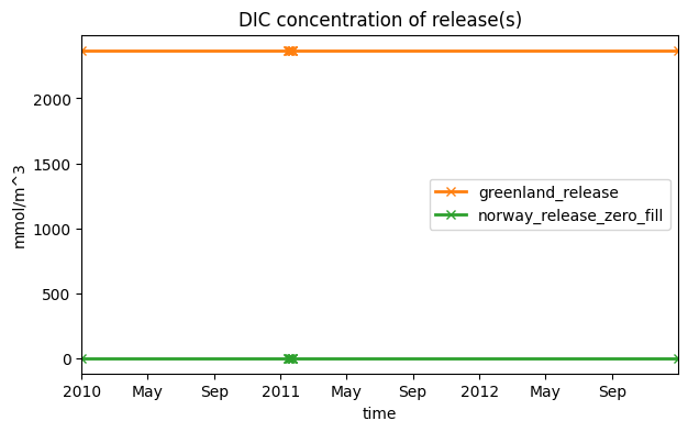
For example, the default values for DIC and PO4 are 2370.0 mmol/m³ and 2.7 mmol/m³, respectively, as can be seen above.
Next, let’s create another release, but this time with fill_values = "zero" to explicitly set all unspecified tracer concentrations to zero.
[8]:
volume_release_norway_with_zero_fill = VolumeRelease(
    name="norway_release_zero_fill",
    lat=65.0,  # degree N
    lon=10,  # degree E
    depth=50,  # m
    times=times,
    volume_fluxes=volume_fluxes,
    tracer_concentrations=tracer_concentrations,
    fill_values="zero",
)
Below, you can see that missing tracer concentrations were correctly set to zero.
[9]:
volume_release_norway_with_zero_fill
[9]:
VolumeRelease(name='norway_release_zero_fill', lat=65.0, lon=10.0, depth=50.0, hsc=0.0, vsc=0.0, times=[datetime.datetime(2011, 1, 15, 12, 0), datetime.datetime(2011, 1, 15, 15, 0), datetime.datetime(2011, 1, 15, 18, 0), datetime.datetime(2011, 1, 19, 0, 0), datetime.datetime(2011, 1, 22, 6, 0), datetime.datetime(2011, 1, 22, 9, 0), datetime.datetime(2011, 1, 22, 12, 0)], time_interpolation=False, release_type=<ReleaseType.volume: 'volume'>, fill_values='zero', volume_fluxes=Flux(name='volume', values=[0.0, 100.0, 500.0, 1000.0, 500.0, 100.0, 0.0]), tracer_concentrations={'ALK': Concentration(name='ALK', values=[1900.0, 2100.0, 2100.0, 2100.0, 2100.0, 2100.0, 1900.0]), 'temp': Concentration(name='temp', values=20.0), 'salt': Concentration(name='salt', values=1.0), 'PO4': Concentration(name='PO4', values=0.0), 'NO3': Concentration(name='NO3', values=0.0), 'SiO3': Concentration(name='SiO3', values=0.0), 'NH4': Concentration(name='NH4', values=0.0), 'Fe': Concentration(name='Fe', values=0.0), 'Lig': Concentration(name='Lig', values=0.0), 'O2': Concentration(name='O2', values=0.0), 'DIC': Concentration(name='DIC', values=0.0), 'DIC_ALT_CO2': Concentration(name='DIC_ALT_CO2', values=0.0), 'ALK_ALT_CO2': Concentration(name='ALK_ALT_CO2', values=0.0), 'DOC': Concentration(name='DOC', values=0.0), 'DON': Concentration(name='DON', values=0.0), 'DOP': Concentration(name='DOP', values=0.0), 'DOPr': Concentration(name='DOPr', values=0.0), 'DONr': Concentration(name='DONr', values=0.0), 'DOCr': Concentration(name='DOCr', values=0.0), 'zooC': Concentration(name='zooC', values=0.0), 'spChl': Concentration(name='spChl', values=0.0), 'spC': Concentration(name='spC', values=0.0), 'spP': Concentration(name='spP', values=0.0), 'spFe': Concentration(name='spFe', values=0.0), 'spCaCO3': Concentration(name='spCaCO3', values=0.0), 'diatChl': Concentration(name='diatChl', values=0.0), 'diatC': Concentration(name='diatC', values=0.0), 'diatP': Concentration(name='diatP', values=0.0), 'diatFe': Concentration(name='diatFe', values=0.0), 'diatSi': Concentration(name='diatSi', values=0.0), 'diazChl': Concentration(name='diazChl', values=0.0), 'diazC': Concentration(name='diazC', values=0.0), 'diazP': Concentration(name='diazP', values=0.0), 'diazFe': Concentration(name='diazFe', values=0.0)})
Note: Later, we’ll cover how to visualize release locations, volume fluxes, and tracer concentrations (including default fill values), once a CDRForcing object has been created.
Defining a TracerPerturbation#
This section covers how to configure and use the TracerPerturbation class to represent injections of tracers without water into a ROMS simulation.
In addition to the location parameters, a TracerPerturbation has the key field:
tracer_fluxes
Both can be specified as either constant or time-varying.
[10]:
from roms_tools import TracerPerturbation
Call .get_metadata() to view the expected units for each tracer flux.
[11]:
TracerPerturbation.get_metadata()
[11]:
| temp | salt | PO4 | NO3 | SiO3 | NH4 | Fe | Lig | O2 | DIC | DIC_ALT_CO2 | ALK | ALK_ALT_CO2 | DOC | DON | DOP | DOPr | DONr | DOCr | zooC | spChl | spC | spP | spFe | spCaCO3 | diatChl | diatC | diatP | diatFe | diatSi | diazChl | diazC | diazP | diazFe | |
|---|---|---|---|---|---|---|---|---|---|---|---|---|---|---|---|---|---|---|---|---|---|---|---|---|---|---|---|---|---|---|---|---|---|---|
| units | degrees Celsius/s | PSU/s | mmol/s | mmol/s | mmol/s | mmol/s | mmol/s | mmol/s | mmol/s | mmol/s | meq/s | meq/s | meq/s | mmol/s | mmol/s | mmol/s | mmol/s | mmol/s | mmol/s | mmol/s | mg/s | mmol/s | mmol/s | mmol/s | mmol/s | mg/s | mmol/s | mmol/s | mmol/s | mmol/s | mg/s | mmol/s | mmol/s | mmol/s |
| long_name | potential temperature | salinity | dissolved inorganic phosphate | dissolved inorganic nitrate | dissolved inorganic silicate | dissolved ammonia | dissolved inorganic iron | iron binding ligand | dissolved oxygen | dissolved inorganic carbon | dissolved inorganic carbon, alternative CO2 | alkalinity | alkalinity, alternative CO2 | dissolved organic carbon | dissolved organic nitrogen | dissolved organic phosphorus | refractory dissolved organic phosphorus | refractory dissolved organic nitrogen | refractory dissolved organic carbon | zooplankton carbon | small phytoplankton chlorophyll | small phytoplankton carbon | small phytoplankton phosphorous | small phytoplankton iron | small phytoplankton CaCO3 | diatom chloropyll | diatom carbon | diatom phosphorus | diatom iron | diatom silicate | diazotroph chloropyll | diazotroph carbon | diazotroph phosphorus | diazotroph iron |
Constant tracer flux#
Let’s start by defining a release near Iceland that has a Gaussian distribution (with standard deviations of 100km in the horizontal and 50m in the vertical) and a constant alkalinity flux:
Alkalinity flux: 2,000,000 meq/s
This ocean alkalinity enhancement (OAE) experiment is equivalent to the VolumeRelease example above, where 2000 meq/m³ of alkalinity was injected with a 1000 m³/s volume flux. However, in this case, no water is added, only the tracer. As before, this single flux value is applied consistently throughout the entire ROMS simulation.
[12]:
constant_oae_iceland = TracerPerturbation(
    name="iceland_oae",
    lat=65.0,  # degree N
    lon=-10,  # degree E
    depth=100,  # m
    hsc=100000,  # m
    vsc=50,  # m
    tracer_fluxes={"ALK": 2 * 10**6},  # meq/s
)
We can also define a direct ocean removal (DOR) experiment as follows.
[13]:
constant_dor_iceland = TracerPerturbation(
    name="iceland_dor",
    lat=65.0,  # degree N
    lon=-25,  # degree E
    depth=100,  # m
    hsc=100000,  # m
    vsc=50,  # m
    tracer_fluxes={"DIC": - 2 * 10**6},  # mmol/s
)
Time-varying tracer fluxes#
To define a time-varying release, specify the times parameter with explicit time points for tracer fluxes.
In the example below, the alkalinity flux varies over time (as list matching times length).
Note
Intermediate tracer flux values between the specified times are linearly interpolated when the CDRForcing object is constructed later.
[14]:
times_trcr = [
    datetime(2011, 1, 15, 12, 0),
    datetime(2011, 1, 15, 15, 0),
    datetime(2011, 1, 15, 18, 0),
    datetime(2011, 1, 19, 0, 0),
    datetime(2011, 1, 22, 6, 0),
    datetime(2011, 1, 22, 9, 0),
    datetime(2011, 1, 22, 12, 0),
]  # 7 entries
tracer_fluxes = {
    "ALK": [
        0.0,
        2.0 * 10**6,  # meq/s
        3.0 * 10**6,  # meq/s
        4.0 * 10**6,  # meq/s
        3.0 * 10**6,  # meq/s
        2.0 * 10**6,  # meq/s
        0.0,
    ],  # 7 entries
}
Given these tracer fluxes, we now define a tracer perturbation as a Gaussian with a standard deviation of 150km in the horizontal and 100m in the vertical.
[15]:
tracer_perturbation_greenland = TracerPerturbation(
    name="greenland_release",
    lat=70.0,  # degree N
    lon=-20.0,  # degree E
    depth=100,  # m
    hsc=150000,  # m
    vsc=100,  # m
    times=times_trcr,
    tracer_fluxes=tracer_fluxes,
)
Fill values are always zero#
For TracerPerturbation, any tracer flux not explicitly specified is automatically set to zero, as this object represents a perturbation rather than a complete tracer field. For that reason, TracerPerturbation does not have a fill_values parameter.
We confirm this automatic zero-filling behavior in the example below.
[16]:
tracer_perturbation_greenland
[16]:
TracerPerturbation(name='greenland_release', lat=70.0, lon=-20.0, depth=100.0, hsc=150000.0, vsc=100.0, times=[datetime.datetime(2011, 1, 15, 12, 0), datetime.datetime(2011, 1, 15, 15, 0), datetime.datetime(2011, 1, 15, 18, 0), datetime.datetime(2011, 1, 19, 0, 0), datetime.datetime(2011, 1, 22, 6, 0), datetime.datetime(2011, 1, 22, 9, 0), datetime.datetime(2011, 1, 22, 12, 0)], time_interpolation=False, release_type=<ReleaseType.tracer_perturbation: 'tracer_perturbation'>, tracer_fluxes={'ALK': Flux(name='ALK', values=[0.0, 2000000.0, 3000000.0, 4000000.0, 3000000.0, 2000000.0, 0.0]), 'temp': Flux(name='temp', values=0.0), 'salt': Flux(name='salt', values=0.0), 'PO4': Flux(name='PO4', values=0.0), 'NO3': Flux(name='NO3', values=0.0), 'SiO3': Flux(name='SiO3', values=0.0), 'NH4': Flux(name='NH4', values=0.0), 'Fe': Flux(name='Fe', values=0.0), 'Lig': Flux(name='Lig', values=0.0), 'O2': Flux(name='O2', values=0.0), 'DIC': Flux(name='DIC', values=0.0), 'DIC_ALT_CO2': Flux(name='DIC_ALT_CO2', values=0.0), 'ALK_ALT_CO2': Flux(name='ALK_ALT_CO2', values=0.0), 'DOC': Flux(name='DOC', values=0.0), 'DON': Flux(name='DON', values=0.0), 'DOP': Flux(name='DOP', values=0.0), 'DOPr': Flux(name='DOPr', values=0.0), 'DONr': Flux(name='DONr', values=0.0), 'DOCr': Flux(name='DOCr', values=0.0), 'zooC': Flux(name='zooC', values=0.0), 'spChl': Flux(name='spChl', values=0.0), 'spC': Flux(name='spC', values=0.0), 'spP': Flux(name='spP', values=0.0), 'spFe': Flux(name='spFe', values=0.0), 'spCaCO3': Flux(name='spCaCO3', values=0.0), 'diatChl': Flux(name='diatChl', values=0.0), 'diatC': Flux(name='diatC', values=0.0), 'diatP': Flux(name='diatP', values=0.0), 'diatFe': Flux(name='diatFe', values=0.0), 'diatSi': Flux(name='diatSi', values=0.0), 'diazChl': Flux(name='diazChl', values=0.0), 'diazC': Flux(name='diazC', values=0.0), 'diazP': Flux(name='diazP', values=0.0), 'diazFe': Flux(name='diazFe', values=0.0)})
CDR Forcing#
The CDR Forcing object links one or multiple releases to the underlying ROMS simulation. It requires the following inputs:
One or multiple releases, all of the same type (either all
VolumeReleaseor allTracerPerturbation)The model grid (optional but strongly recommended)
The simulation start and end dates (required)
Notes
Model Grid: Although optional, providing the model grid is highly recommended. Without it, important validation checks, such as verifying whether release locations fall outside the grid domain or on land, cannot be performed. Additionally, plotting release locations requires the model grid to be provided.
Simulation Start and End Dates: These are necessary for two reasons:
To ensure that the release window does not fall outside the simulation window.
ROMS requires forcing data for the entire simulation period. If a release’s specified times do not fully cover the simulation period, ROMS-Tools will extend the release data to the simulation endpoints using a default method (details provided in this section).
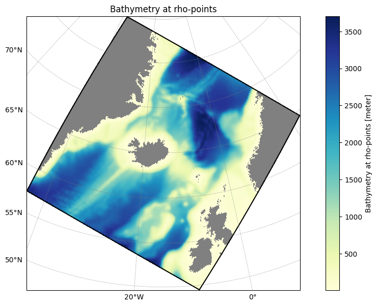
Let’s create our CDR forcings for the following grid spanning the Nordic Seas.
[17]:
from roms_tools import Grid
[18]:
grid = Grid(
    nx=250,
    ny=250,
    size_x=2500,
    size_y=2500,
    center_lon=-15,
    center_lat=65,
    rot=-30,
    N=100,
    topography_source={
        "name": "SRTM15",
        "path": "/anvil/projects/x-ees250129/Datasets/SRTM15/SRTM15_V2.6.nc",
    },
)
[19]:
grid.plot()
Next, we specify the start and end times of the underlying ROMS simulation.
[20]:
simulation_start_time = datetime(2010, 1, 1)
simulation_end_time = datetime(2012, 12, 31)
Creating the CDRForcing#
[21]:
simulation_end_time-simulation_start_time
[21]:
datetime.timedelta(days=1095)
[22]:
from roms_tools import CDRForcing
Let’s first create a CDRForcing that consists of all the VolumeReleases that we defined above.
[23]:
cdr_forcing_with_volume_releases = CDRForcing(
    grid=grid,
    start_time=simulation_start_time,
    end_time=simulation_end_time,
    model_reference_date=datetime(2000, 1, 1), # this is the default
    releases=[
        constant_volume_release_iceland,
        volume_release_greenland,
        volume_release_norway_with_zero_fill,
    ],
)
Similarly, we can create a CDRForcing that consists of all the TracerPerturbations that we defined above.
[24]:
cdr_forcing_with_tracer_perturbations = CDRForcing(
    grid=grid,
    start_time=simulation_start_time,
    end_time=simulation_end_time,
    model_reference_date=datetime(2000, 1, 1), # this is the default
    releases=[
        constant_oae_iceland,
        constant_dor_iceland,
        tracer_perturbation_greenland,
    ],
)
The .ds attribute of each CDRForcing object holds an xarray Dataset with the release information. This dataset can eventually be saved to a NetCDF file, providing the ROMS input file.
[25]:
cdr_forcing_with_volume_releases.ds
[25]:
<xarray.Dataset> Size: 17kB
Dimensions:           (time: 9, ncdr: 3, ntracers: 34)
Coordinates:
  * time              (time) datetime64[ns] 72B 2010-01-01 ... 2012-12-31
    release_name      (ncdr) <U24 288B 'iceland_release' ... 'norway_release_...
    tracer_name       (ntracers) <U11 1kB 'temp' 'salt' ... 'diazP' 'diazFe'
    tracer_unit       (ntracers) <U15 2kB 'degrees Celsius' 'PSU' ... 'mmol/m^3'
    tracer_long_name  (ntracers) <U43 6kB 'potential temperature' ... 'diazot...
Dimensions without coordinates: ncdr, ntracers
Data variables:
    cdr_time          (time) float64 72B 3.653e+03 4.032e+03 ... 4.748e+03
    cdr_lon           (ncdr) float64 24B -10.0 -20.0 10.0
    cdr_lat           (ncdr) float64 24B 65.0 70.0 65.0
    cdr_dep           (ncdr) float64 24B 100.0 100.0 50.0
    cdr_hsc           (ncdr) float64 24B 0.0 0.0 0.0
    cdr_vsc           (ncdr) float64 24B 0.0 0.0 0.0
    cdr_interp        (ncdr) bool 3B False False False
    cdr_volume        (time, ncdr) float64 216B 1e+03 0.0 0.0 ... 1e+03 0.0 0.0
cdr_tracer (time, ntracers, ncdr) float64 7kB 20.0 20.0 ... 0.0The dataset above contains 3 releases, as indicated by the ncdr dimension.
In contrast, the next dataset contains only 2 releases, as expected.
[26]:
cdr_forcing_with_tracer_perturbations.ds
[26]:
<xarray.Dataset> Size: 17kB
Dimensions:           (time: 9, ncdr: 3, ntracers: 34)
Coordinates:
  * time              (time) datetime64[ns] 72B 2010-01-01 ... 2012-12-31
    release_name      (ncdr) <U17 204B 'iceland_oae' ... 'greenland_release'
    tracer_name       (ntracers) <U11 1kB 'temp' 'salt' ... 'diazP' 'diazFe'
    tracer_unit       (ntracers) <U17 2kB 'degrees Celsius/s' ... 'mmol/s'
    tracer_long_name  (ntracers) <U43 6kB 'potential temperature' ... 'diazot...
Dimensions without coordinates: ncdr, ntracers
Data variables:
    cdr_time          (time) float64 72B 3.653e+03 4.032e+03 ... 4.748e+03
    cdr_lon           (ncdr) float64 24B -10.0 -25.0 -20.0
    cdr_lat           (ncdr) float64 24B 65.0 65.0 70.0
    cdr_dep           (ncdr) float64 24B 100.0 100.0 100.0
    cdr_hsc           (ncdr) float64 24B 1e+05 1e+05 1.5e+05
    cdr_vsc           (ncdr) float64 24B 50.0 50.0 100.0
    cdr_interp        (ncdr) bool 3B False False False
cdr_trcflx (time, ntracers, ncdr) float64 7kB 0.0 0.0 0.0 ... 0.0 0.0Plotting the Release Locations and Distributions#
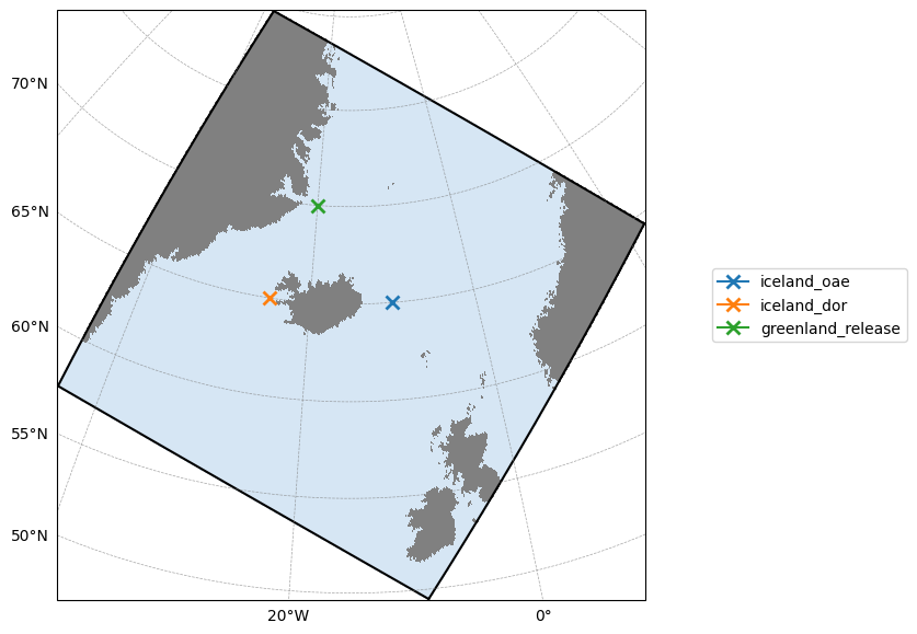
We now continue with visualizing the release locations and distributions. First, we will create a bird’s-eye view of the release location centers.
[27]:
cdr_forcing_with_volume_releases.plot_locations() # By default, this plots all available releases (but max 20).
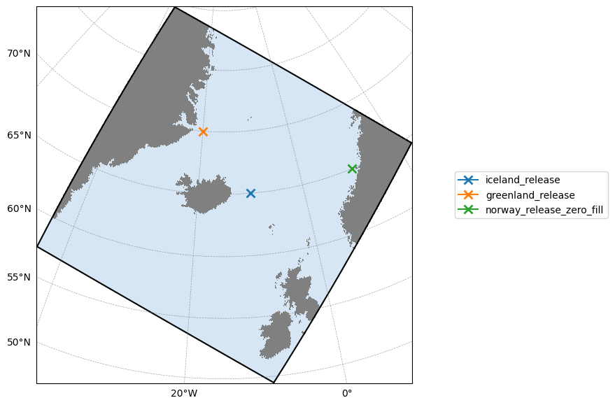
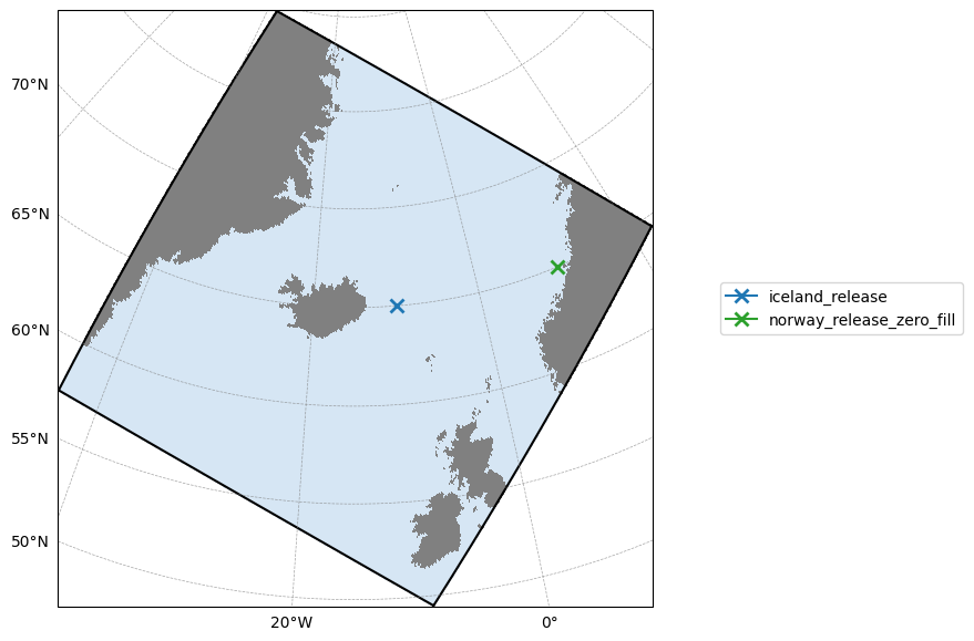
We can also restrict the plot to display only the releases of interest by specifying them in a list via the release_names parameter.
[28]:
cdr_forcing_with_volume_releases.plot_locations(
    release_names=["iceland_release", "norway_release_zero_fill"]
)
[29]:
cdr_forcing_with_tracer_perturbations.plot_locations()
Next, we plot the release distributions from a top and side view. Note that we can only plot one release at a time in this view, as the latitude and longitude section to be visualized depends on the specific location of the release itself.
[30]:
cdr_forcing_with_volume_releases.plot_distribution(release_name="greenland_release")
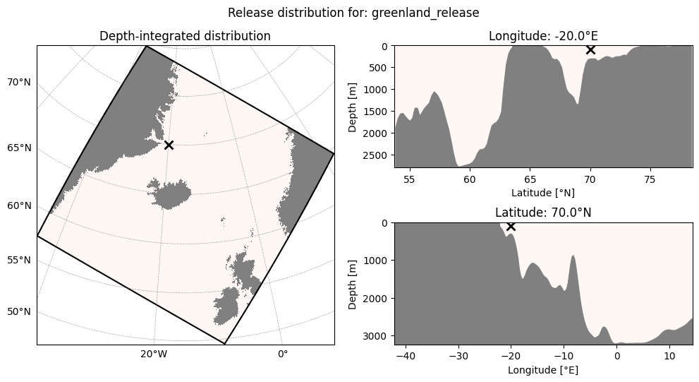
The VolumeRelease we visualized in the plot above is a point source. Next, let’s visualize our tracer perturbations, which are released as Gaussian distributions.
[31]:
cdr_forcing_with_tracer_perturbations.plot_distribution(
    release_name="greenland_release"
)
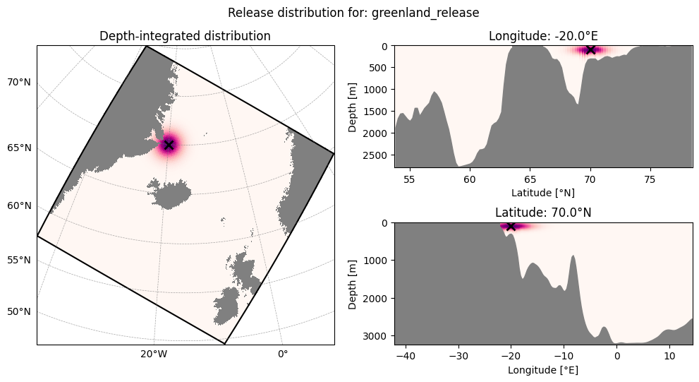
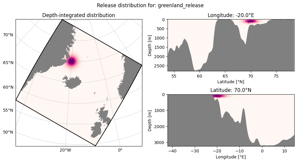
If the black cross at the release center bothers you, you can remove it by setting mark_release_center = False, as shown in the next plot.
[32]:
cdr_forcing_with_tracer_perturbations.plot_distribution(
    release_name="greenland_release", mark_release_center=False
)
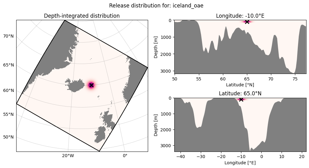
[33]:
cdr_forcing_with_tracer_perturbations.plot_distribution(release_name="iceland_oae")
Plotting Volume Fluxes and Tracer Concentrations#
This section applies only to CDRForcing objects that contain releases of type VolumeRelease. These releases are associated with both volume fluxes and tracer concentrations, which we will visualize next.
[34]:
cdr_forcing_with_volume_releases.plot_volume_flux()
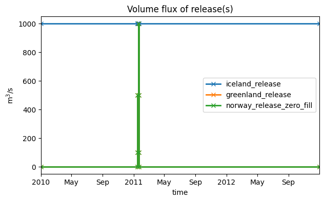
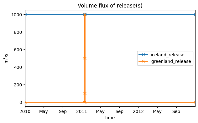
You can see that the iceland_release applies a constant volume flux throughout the entire simulation period, while the other two releases have time-varying volume fluxes, just as we designed them earlier.
If desired, you can also limit the plot to specific releases using the release_names parameter.
[35]:
cdr_forcing_with_volume_releases.plot_volume_flux(
    release_names=["iceland_release", "greenland_release"]
)
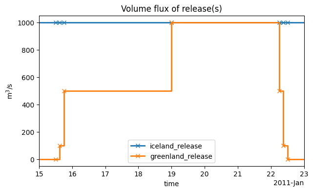
We can also zoom into the specific time window where the greenland_release occurs to better visualize the time-varying behavior of the volume flux.
[36]:
cdr_forcing_with_volume_releases.plot_volume_flux(
    release_names=["iceland_release", "greenland_release"],
    start=datetime(2011, 1, 15),
    end=datetime(2011, 1, 23),
)
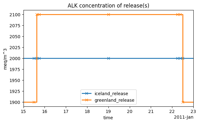
Next, we plot the alkalinity concentration.
[37]:
cdr_forcing_with_volume_releases.plot_tracer_concentration(
    tracer_name="ALK", release_names=["iceland_release", "greenland_release"]
)
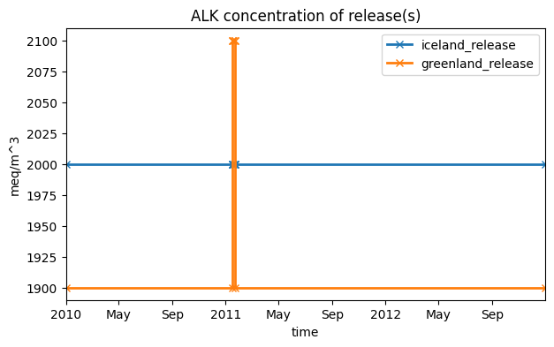
Again, the iceland_release uses an alkalinity concentration that is constant in time, while the greenland_release has a time-varying alkalinity concentration.
[38]:
cdr_forcing_with_volume_releases.plot_tracer_concentration(
    tracer_name="ALK",
    release_names=["iceland_release", "greenland_release"],
    start=datetime(2011, 1, 15),
    end=datetime(2011, 1, 23),
)
Finally, we plot the DIC concentration to visualize the effect of the default fill versus the zero fill.
[39]:
cdr_forcing_with_volume_releases.plot_tracer_concentration(
    tracer_name="DIC", release_names=["greenland_release", "norway_release_zero_fill"]
)
Plotting Tracer Fluxes#
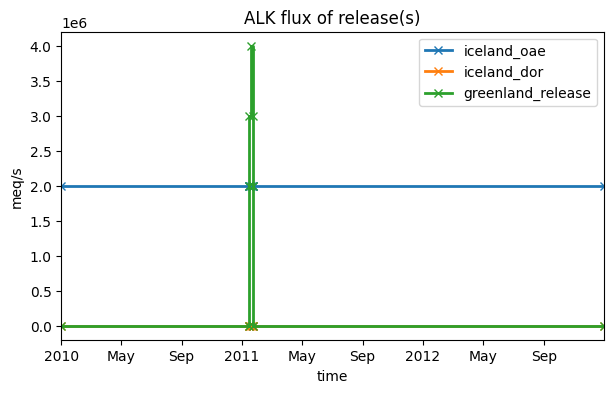
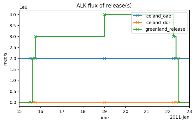
This section applies only to CDRForcing objects that contain releases of type TracerPerturbation. These releases are associated with tracer fluxes, which we will visualize next. The plot_tracer_flux method works similarly as the plot_volume_flux and plot_tracer_concentration methods above.
[40]:
cdr_forcing_with_tracer_perturbations.plot_tracer_flux(tracer_name="ALK")
[41]:
cdr_forcing_with_tracer_perturbations.plot_tracer_flux(
    tracer_name="ALK", start=datetime(2011, 1, 15), end=datetime(2011, 1, 23)
)
[42]:
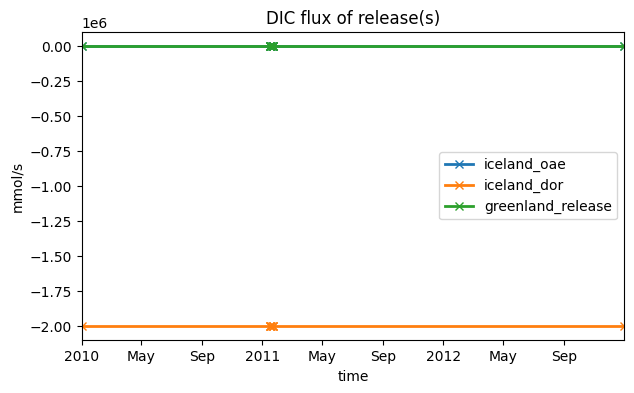
cdr_forcing_with_tracer_perturbations.plot_tracer_flux(tracer_name="DIC")
Linear Interpolation#
So far, all of our volume flux and tracer concentrations have been shown as step function, where the value stays constant until a new value is prescribed. This is because CDRForcing sets time_interpolation to False by default. If we want to interpolate between points, we can set it to True.
Let’s remake our previous example volume_release_greenland, but setting time_interpolation=True.
[43]:
volume_release_greenland_interpolation = VolumeRelease(
    name="greenland_release",
    lat=70.0,  # degree N
    lon=-20.0,  # degree E
    depth=100,  # m
    times=volume_release_greenland.times,
    volume_fluxes=volume_release_greenland.volume_fluxes.values,
    tracer_concentrations=volume_release_greenland.tracer_concentrations,
    time_interpolation=True,
)

cdr_forcing_with_volume_release_interpolation = CDRForcing(
    grid=grid,
    start_time=simulation_start_time,
    end_time=simulation_end_time,
    model_reference_date=datetime(2000, 1, 1), # this is the default
    releases=[
        volume_release_greenland_interpolation,
    ],
)
[44]:
cdr_forcing_with_volume_release_interpolation.plot_volume_flux(
    release_names=["greenland_release"],
    start=datetime(2011, 1, 15),
    end=datetime(2011, 1, 23),
)
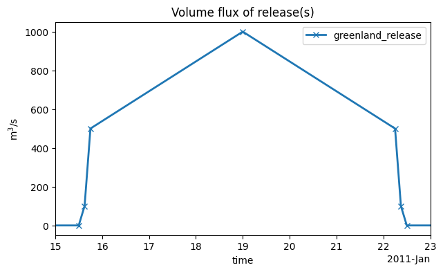
Notice how there is a tail between the start time (datetime(2010, 1, 1)) and our first assigned date (datetime(2011, 1, 15, 12, 0)). This is due to the automatic extrapolation that ROMS-Tools performs.
Automatic Extrapolation to Simulation Endpoints#
Important
ROMS requires volume fluxes and tracer concentrations for the entire simulation period. If the user does not specify the simulation’s start and end points in their time series, ROMS-Tools will apply the following defaults:
Volume and tracer fluxes are set to 0 at both the start and end times.
Tracer concentrations at the start and end times are set to the values from the closest available time stamps.
Let’s examine how these rules play out in practice by revisiting our previous VolumeRelease examples: volume_release_greenland_interpolation. This release was defined with the following times, volume fluxes, and alkalinity concentrations (where the endpoints have been filled in when we built cdr_forcing_with_volume_release_interpolation).
[45]:
volume_release_greenland_interpolation.times
[45]:
[datetime.datetime(2010, 1, 1, 0, 0),
 datetime.datetime(2011, 1, 15, 12, 0),
 datetime.datetime(2011, 1, 15, 15, 0),
 datetime.datetime(2011, 1, 15, 18, 0),
 datetime.datetime(2011, 1, 19, 0, 0),
 datetime.datetime(2011, 1, 22, 6, 0),
 datetime.datetime(2011, 1, 22, 9, 0),
 datetime.datetime(2011, 1, 22, 12, 0),
 datetime.datetime(2012, 12, 31, 0, 0)]
[46]:
volume_release_greenland_interpolation.volume_fluxes.values
[46]:
[0.0, 0.0, 100.0, 500.0, 1000.0, 500.0, 100.0, 0.0, 0.0]
[47]:
volume_release_greenland_interpolation.tracer_concentrations["ALK"].values
[47]:
[1900.0, 1900.0, 2100.0, 2100.0, 2100.0, 2100.0, 2100.0, 1900.0, 1900.0]
In the next example, we define a very similar release as before, but we omit the first two and the last two timestamps from the time series.
[48]:
times = volume_release_greenland_interpolation.times[2:-2]
times
[48]:
[datetime.datetime(2011, 1, 15, 15, 0),
 datetime.datetime(2011, 1, 15, 18, 0),
 datetime.datetime(2011, 1, 19, 0, 0),
 datetime.datetime(2011, 1, 22, 6, 0),
 datetime.datetime(2011, 1, 22, 9, 0)]
[49]:
volume_fluxes = volume_release_greenland_interpolation.volume_fluxes.values[2:-2]
volume_fluxes
[49]:
[100.0, 500.0, 1000.0, 500.0, 100.0]
[50]:
alk_concentration = volume_release_greenland_interpolation.tracer_concentrations["ALK"].values[2:-2]
alk_concentration
[50]:
[2100.0, 2100.0, 2100.0, 2100.0, 2100.0]
[51]:
volume_release_greenland_interpolation_truncated = VolumeRelease(
    name="greenland_release_cut_short",
    lat=volume_release_greenland.lat,
    lon=volume_release_greenland.lon,
    depth=volume_release_greenland.depth,
    times=times,
    volume_fluxes=volume_fluxes,
    tracer_concentrations={"ALK": alk_concentration},
    time_interpolation=True,
)
[52]:
volume_release_greenland_interpolation_truncated.volume_fluxes.values
[52]:
[100.0, 500.0, 1000.0, 500.0, 100.0]
[53]:
cdr_forcing = CDRForcing(
    grid=grid,
    start_time=simulation_start_time,
    end_time=simulation_end_time,
    releases=[volume_release_greenland_interpolation, volume_release_greenland_interpolation_truncated],
)
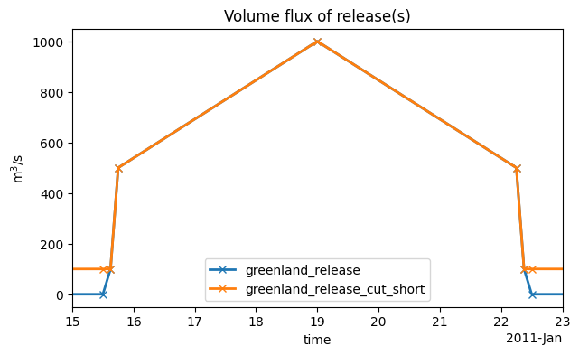
Let’s now compare the time series of volume flux and alkalinity concentration for the two releases.
[54]:
cdr_forcing.plot_volume_flux(start=datetime(2011, 1, 15), end=datetime(2011, 1, 23))
If we zoom out, we can see how the tails are handled.
[55]:
cdr_forcing.plot_volume_flux()
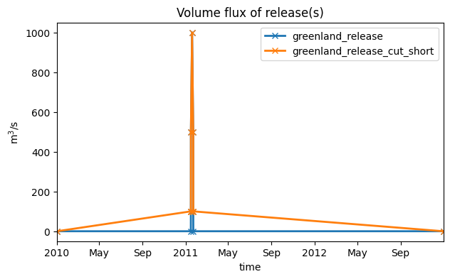
We see that when time_interpolation is turned on, not assigning values to the start and end points on the simulation will result in ROMS-Tools extrapolating to 0 for each. Explicitly prescribing times when the volume and tracer fluxes avoids this tail of additional fluxes.
To re-iterate, the above plot shows the effect of choosing:
volume_fluxes = [0.0, 100.0, 500.0, 1000.0, 500.0, 100.0, 0.0](blue line) vs.volume_fluxes = [100.0, 500.0, 1000.0, 500.0, 100.0](orange line)
ROMS-Tools assumes the flux is only shut off at the simulation endpoints and linearly interpolates in between.[56]:
cdr_forcing.plot_tracer_concentration(tracer_name="ALK")
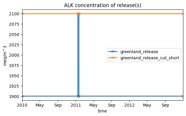
To re-iterate, the above plot shows the effect of choosing:
tracer_concentrations["ALK"] = [1900.0, 2100.0, 2100.0, 2100.0, 2100.0, 2100.0, 1900.0](blue line) vs.tracer_concentrations["ALK"] = [2100.0, 2100.0, 2100.0, 2100.0, 2100.0](orange line)
In both cases, ROMS-Tools extrapolates the endpoints of the provided time series to the simulation endpoints.
Total Tracer Release Accounting#
In marine CDR experiments, it is essential to ensure that the ROMS simulation matches the intended tracer inputs, e.g., the total amount of alkalinity added or DIC removed. To achieve this, ROMS-Tools computes the cumulative tracer release for each release over the simulation period via the .compute_total_cdr_source() method.
The total amount of tracer released or removed depends on the time discretization used in the ROMS simulation. To reproduce exactly what ROMS will do, ROMS-Tools reconstructs the ROMS time stamps. This requires:
The simulation start and end times, already provided when instantiating the CDRForcing object (
start_timeandend_time). Make sure that these exactly match the actual start and end time of the simulation.The model time step
dt, which defines the temporal resolution of the integration.
The output is a pandas DataFrame with releases as rows and tracers as columns, showing the cumulative mass of each tracer released. Different choices of dt may produce slightly different totals due to discretization.
[57]:
dt0 = 150 # ROMS time step in seconds
df0_vr = cdr_forcing_with_volume_releases.compute_total_cdr_source(dt=dt0)
df0_vr
[57]:
| ALK | PO4 | NO3 | SiO3 | NH4 | Fe | Lig | O2 | DIC | DIC_ALT_CO2 | ALK_ALT_CO2 | DOC | DON | DOP | DOPr | DONr | DOCr | zooC | spChl | spC | spP | spFe | spCaCO3 | diatChl | diatC | diatP | diatFe | diatSi | diazChl | diazC | diazP | diazFe | |
|---|---|---|---|---|---|---|---|---|---|---|---|---|---|---|---|---|---|---|---|---|---|---|---|---|---|---|---|---|---|---|---|---|
| units | meq | mmol | mmol | mmol | mmol | mmol | mmol | mmol | mmol | meq | meq | mmol | mmol | mmol | mmol | mmol | mmol | mmol | mg | mmol | mmol | mmol | mmol | mg | mmol | mmol | mmol | mmol | mg | mmol | mmol | mmol |
| iceland_release | 189216000000000.0 | 255441600000.0 | 2289513600000.0 | 1248825600000.0 | 208137600000.0 | 169348320000.0 | 508044960000.0 | 17739000000000.0 | 224220960000000.0 | 224220960000000.0 | 218544480000000.0 | 9460800.0 | 94608000000.0 | 9460800000.0 | 283824000.0 | 75686400000.0 | 94608.0 | 255441600000.0 | 127720800000.0 | 638604000000.0 | 4257360000.0 | 2554416.0 | 12772080000.0 | 12772080000.0 | 38316240000.0 | 2838240000.0 | 255441.6 | 12772080000.0 | 1419120000.0 | 7095600000.0 | 1419120000.0 | 141912.0 |
| greenland_release | 900396000000.0 | 1157652000.0 | 10375992000.0 | 5659632000.0 | 943272000.0 | 767480400.0 | 2302441200.0 | 80392500000.0 | 1016161200000.0 | 1016161200000.0 | 990435600000.0 | 42876.0 | 428760000.0 | 42876000.0 | 1286280.0 | 343008000.0 | 428.76 | 1157652000.0 | 578826000.0 | 2894130000.0 | 19294200.0 | 11576.52 | 57882600.0 | 57882600.0 | 173647800.0 | 12862800.0 | 1157.652 | 57882600.0 | 6431400.0 | 32157000.0 | 6431400.0 | 643.14 |
| norway_release_zero_fill | 900396000000.0 | 0.0 | 0.0 | 0.0 | 0.0 | 0.0 | 0.0 | 0.0 | 0.0 | 0.0 | 0.0 | 0.0 | 0.0 | 0.0 | 0.0 | 0.0 | 0.0 | 0.0 | 0.0 | 0.0 | 0.0 | 0.0 | 0.0 | 0.0 | 0.0 | 0.0 | 0.0 | 0.0 | 0.0 | 0.0 | 0.0 | 0.0 |
We can do a similar analysis for our released tracer perturbations.
[58]:
df0_tp = cdr_forcing_with_tracer_perturbations.compute_total_cdr_source(dt=150)
df0_tp
[58]:
| ALK | PO4 | NO3 | SiO3 | NH4 | Fe | Lig | O2 | DIC | DIC_ALT_CO2 | ALK_ALT_CO2 | DOC | DON | DOP | DOPr | DONr | DOCr | zooC | spChl | spC | spP | spFe | spCaCO3 | diatChl | diatC | diatP | diatFe | diatSi | diazChl | diazC | diazP | diazFe | |
|---|---|---|---|---|---|---|---|---|---|---|---|---|---|---|---|---|---|---|---|---|---|---|---|---|---|---|---|---|---|---|---|---|
| units | meq | mmol | mmol | mmol | mmol | mmol | mmol | mmol | mmol | meq | meq | mmol | mmol | mmol | mmol | mmol | mmol | mmol | mg | mmol | mmol | mmol | mmol | mg | mmol | mmol | mmol | mmol | mg | mmol | mmol | mmol |
| iceland_oae | 189216000000000.0 | 0.0 | 0.0 | 0.0 | 0.0 | 0.0 | 0.0 | 0.0 | 0.0 | 0.0 | 0.0 | 0.0 | 0.0 | 0.0 | 0.0 | 0.0 | 0.0 | 0.0 | 0.0 | 0.0 | 0.0 | 0.0 | 0.0 | 0.0 | 0.0 | 0.0 | 0.0 | 0.0 | 0.0 | 0.0 | 0.0 | 0.0 |
| iceland_dor | 0.0 | 0.0 | 0.0 | 0.0 | 0.0 | 0.0 | 0.0 | 0.0 | -189216000000000.0 | 0.0 | 0.0 | 0.0 | 0.0 | 0.0 | 0.0 | 0.0 | 0.0 | 0.0 | 0.0 | 0.0 | 0.0 | 0.0 | 0.0 | 0.0 | 0.0 | 0.0 | 0.0 | 0.0 | 0.0 | 0.0 | 0.0 | 0.0 |
| greenland_release | 2041200000000.0 | 0.0 | 0.0 | 0.0 | 0.0 | 0.0 | 0.0 | 0.0 | 0.0 | 0.0 | 0.0 | 0.0 | 0.0 | 0.0 | 0.0 | 0.0 | 0.0 | 0.0 | 0.0 | 0.0 | 0.0 | 0.0 | 0.0 | 0.0 | 0.0 | 0.0 | 0.0 | 0.0 | 0.0 | 0.0 | 0.0 | 0.0 |
Saving as NetCDF or YAML File#
We can now save our CDR forcing data as a NetCDF file using the .save method. This file will include the dataset stored in .ds. The resulting NetCDF file can then be used as input for ROMS simulations.
In this example, we focus on the CDR forcing built from VolumeRelease objects, but the same saving procedure applies to CDR forcing created from TracerPerturbation objects.
[59]:
filepath = "my_cdr_forcing.nc"
[60]:
cdr_forcing_with_volume_releases.save(filepath=filepath)
2026-05-11 19:40:40 - INFO - Writing the following NetCDF files:
my_cdr_forcing.nc
[60]:
[PosixPath('my_cdr_forcing.nc')]
We can also export the CDR forcing parameters and their associated release information to a YAML file.
[61]:
yaml_filepath = "my_cdr_forcing.yaml"
[62]:
cdr_forcing_with_volume_releases.to_yaml(yaml_filepath)
This is the YAML file that was created.
[63]:
# Open and read the YAML file
with open(yaml_filepath, "r") as file:
    file_contents = file.read()

# Print the contents
print(file_contents)
---
roms_tools_version: 3.6.1.dev31+g34326e51e
---
Grid:
nx: 250
ny: 250
size_x: 2500
size_y: 2500
center_lon: -15
center_lat: 65
rot: -30
N: 100
theta_s: 5.0
theta_b: 2.0
hc: 300.0
topography_source:
name: SRTM15
path: /anvil/projects/x-ees250129/Datasets/SRTM15/SRTM15_V2.6.nc
mask_shapefile: null
close_narrow_channels: false
hmin: 5.0
filename: null
CDRForcing:
start_time: '2010-01-01T00:00:00'
end_time: '2012-12-31T00:00:00'
model_reference_date: '2000-01-01T00:00:00'
releases:
- name: iceland_release
lat: 65.0
lon: -10.0
depth: 100.0
hsc: 0.0
vsc: 0.0
times:
- 2010-01-01 00:00:00
- 2012-12-31 00:00:00
time_interpolation: false
release_type: volume
fill_values: auto
volume_fluxes:
- 1000.0
- 1000.0
tracer_concentrations:
temp:
- 20.0
- 20.0
salt:
- 1.0
- 1.0
ALK:
- 2000.0
- 2000.0
PO4:
- 2.7
- 2.7
NO3:
- 24.2
- 24.2
SiO3:
- 13.2
- 13.2
NH4:
- 2.2
- 2.2
Fe:
- 1.79
- 1.79
Lig:
- 5.37
- 5.37
O2:
- 187.5
- 187.5
DIC:
- 2370.0
- 2370.0
DIC_ALT_CO2:
- 2370.0
- 2370.0
ALK_ALT_CO2:
- 2310.0
- 2310.0
DOC:
- 0.0001
- 0.0001
DON:
- 1.0
- 1.0
DOP:
- 0.1
- 0.1
DOPr:
- 0.003
- 0.003
DONr:
- 0.8
- 0.8
DOCr:
- 1.0e-06
- 1.0e-06
zooC:
- 2.7
- 2.7
spChl:
- 1.35
- 1.35
spC:
- 6.75
- 6.75
spP:
- 0.045
- 0.045
spFe:
- 2.7e-05
- 2.7e-05
spCaCO3:
- 0.135
- 0.135
diatChl:
- 0.135
- 0.135
diatC:
- 0.405
- 0.405
diatP:
- 0.03
- 0.03
diatFe:
- 2.7e-06
- 2.7e-06
diatSi:
- 0.135
- 0.135
diazChl:
- 0.015
- 0.015
diazC:
- 0.075
- 0.075
diazP:
- 0.015
- 0.015
diazFe:
- 1.5e-06
- 1.5e-06
- name: greenland_release
lat: 70.0
lon: -20.0
depth: 100.0
hsc: 0.0
vsc: 0.0
times:
- 2010-01-01 00:00:00
- 2011-01-15 12:00:00
- 2011-01-15 15:00:00
- 2011-01-15 18:00:00
- 2011-01-19 00:00:00
- 2011-01-22 06:00:00
- 2011-01-22 09:00:00
- 2011-01-22 12:00:00
- 2012-12-31 00:00:00
time_interpolation: false
release_type: volume
fill_values: auto
volume_fluxes:
- 0.0
- 0.0
- 100.0
- 500.0
- 1000.0
- 500.0
- 100.0
- 0.0
- 0.0
tracer_concentrations:
ALK:
- 1900.0
- 1900.0
- 2100.0
- 2100.0
- 2100.0
- 2100.0
- 2100.0
- 1900.0
- 1900.0
temp:
- 20.0
- 20.0
- 20.0
- 20.0
- 20.0
- 20.0
- 20.0
- 20.0
- 20.0
salt:
- 1.0
- 1.0
- 1.0
- 1.0
- 1.0
- 1.0
- 1.0
- 1.0
- 1.0
PO4:
- 2.7
- 2.7
- 2.7
- 2.7
- 2.7
- 2.7
- 2.7
- 2.7
- 2.7
NO3:
- 24.2
- 24.2
- 24.2
- 24.2
- 24.2
- 24.2
- 24.2
- 24.2
- 24.2
SiO3:
- 13.2
- 13.2
- 13.2
- 13.2
- 13.2
- 13.2
- 13.2
- 13.2
- 13.2
NH4:
- 2.2
- 2.2
- 2.2
- 2.2
- 2.2
- 2.2
- 2.2
- 2.2
- 2.2
Fe:
- 1.79
- 1.79
- 1.79
- 1.79
- 1.79
- 1.79
- 1.79
- 1.79
- 1.79
Lig:
- 5.37
- 5.37
- 5.37
- 5.37
- 5.37
- 5.37
- 5.37
- 5.37
- 5.37
O2:
- 187.5
- 187.5
- 187.5
- 187.5
- 187.5
- 187.5
- 187.5
- 187.5
- 187.5
DIC:
- 2370.0
- 2370.0
- 2370.0
- 2370.0
- 2370.0
- 2370.0
- 2370.0
- 2370.0
- 2370.0
DIC_ALT_CO2:
- 2370.0
- 2370.0
- 2370.0
- 2370.0
- 2370.0
- 2370.0
- 2370.0
- 2370.0
- 2370.0
ALK_ALT_CO2:
- 2310.0
- 2310.0
- 2310.0
- 2310.0
- 2310.0
- 2310.0
- 2310.0
- 2310.0
- 2310.0
DOC:
- 0.0001
- 0.0001
- 0.0001
- 0.0001
- 0.0001
- 0.0001
- 0.0001
- 0.0001
- 0.0001
DON:
- 1.0
- 1.0
- 1.0
- 1.0
- 1.0
- 1.0
- 1.0
- 1.0
- 1.0
DOP:
- 0.1
- 0.1
- 0.1
- 0.1
- 0.1
- 0.1
- 0.1
- 0.1
- 0.1
DOPr:
- 0.003
- 0.003
- 0.003
- 0.003
- 0.003
- 0.003
- 0.003
- 0.003
- 0.003
DONr:
- 0.8
- 0.8
- 0.8
- 0.8
- 0.8
- 0.8
- 0.8
- 0.8
- 0.8
DOCr:
- 1.0e-06
- 1.0e-06
- 1.0e-06
- 1.0e-06
- 1.0e-06
- 1.0e-06
- 1.0e-06
- 1.0e-06
- 1.0e-06
zooC:
- 2.7
- 2.7
- 2.7
- 2.7
- 2.7
- 2.7
- 2.7
- 2.7
- 2.7
spChl:
- 1.35
- 1.35
- 1.35
- 1.35
- 1.35
- 1.35
- 1.35
- 1.35
- 1.35
spC:
- 6.75
- 6.75
- 6.75
- 6.75
- 6.75
- 6.75
- 6.75
- 6.75
- 6.75
spP:
- 0.045
- 0.045
- 0.045
- 0.045
- 0.045
- 0.045
- 0.045
- 0.045
- 0.045
spFe:
- 2.7e-05
- 2.7e-05
- 2.7e-05
- 2.7e-05
- 2.7e-05
- 2.7e-05
- 2.7e-05
- 2.7e-05
- 2.7e-05
spCaCO3:
- 0.135
- 0.135
- 0.135
- 0.135
- 0.135
- 0.135
- 0.135
- 0.135
- 0.135
diatChl:
- 0.135
- 0.135
- 0.135
- 0.135
- 0.135
- 0.135
- 0.135
- 0.135
- 0.135
diatC:
- 0.405
- 0.405
- 0.405
- 0.405
- 0.405
- 0.405
- 0.405
- 0.405
- 0.405
diatP:
- 0.03
- 0.03
- 0.03
- 0.03
- 0.03
- 0.03
- 0.03
- 0.03
- 0.03
diatFe:
- 2.7e-06
- 2.7e-06
- 2.7e-06
- 2.7e-06
- 2.7e-06
- 2.7e-06
- 2.7e-06
- 2.7e-06
- 2.7e-06
diatSi:
- 0.135
- 0.135
- 0.135
- 0.135
- 0.135
- 0.135
- 0.135
- 0.135
- 0.135
diazChl:
- 0.015
- 0.015
- 0.015
- 0.015
- 0.015
- 0.015
- 0.015
- 0.015
- 0.015
diazC:
- 0.075
- 0.075
- 0.075
- 0.075
- 0.075
- 0.075
- 0.075
- 0.075
- 0.075
diazP:
- 0.015
- 0.015
- 0.015
- 0.015
- 0.015
- 0.015
- 0.015
- 0.015
- 0.015
diazFe:
- 1.5e-06
- 1.5e-06
- 1.5e-06
- 1.5e-06
- 1.5e-06
- 1.5e-06
- 1.5e-06
- 1.5e-06
- 1.5e-06
- name: norway_release_zero_fill
lat: 65.0
lon: 10.0
depth: 50.0
hsc: 0.0
vsc: 0.0
times:
- 2010-01-01 00:00:00
- 2011-01-15 12:00:00
- 2011-01-15 15:00:00
- 2011-01-15 18:00:00
- 2011-01-19 00:00:00
- 2011-01-22 06:00:00
- 2011-01-22 09:00:00
- 2011-01-22 12:00:00
- 2012-12-31 00:00:00
time_interpolation: false
release_type: volume
fill_values: zero
volume_fluxes:
- 0.0
- 0.0
- 100.0
- 500.0
- 1000.0
- 500.0
- 100.0
- 0.0
- 0.0
tracer_concentrations:
ALK:
- 1900.0
- 1900.0
- 2100.0
- 2100.0
- 2100.0
- 2100.0
- 2100.0
- 1900.0
- 1900.0
temp:
- 20.0
- 20.0
- 20.0
- 20.0
- 20.0
- 20.0
- 20.0
- 20.0
- 20.0
salt:
- 1.0
- 1.0
- 1.0
- 1.0
- 1.0
- 1.0
- 1.0
- 1.0
- 1.0
PO4:
- 0.0
- 0.0
- 0.0
- 0.0
- 0.0
- 0.0
- 0.0
- 0.0
- 0.0
NO3:
- 0.0
- 0.0
- 0.0
- 0.0
- 0.0
- 0.0
- 0.0
- 0.0
- 0.0
SiO3:
- 0.0
- 0.0
- 0.0
- 0.0
- 0.0
- 0.0
- 0.0
- 0.0
- 0.0
NH4:
- 0.0
- 0.0
- 0.0
- 0.0
- 0.0
- 0.0
- 0.0
- 0.0
- 0.0
Fe:
- 0.0
- 0.0
- 0.0
- 0.0
- 0.0
- 0.0
- 0.0
- 0.0
- 0.0
Lig:
- 0.0
- 0.0
- 0.0
- 0.0
- 0.0
- 0.0
- 0.0
- 0.0
- 0.0
O2:
- 0.0
- 0.0
- 0.0
- 0.0
- 0.0
- 0.0
- 0.0
- 0.0
- 0.0
DIC:
- 0.0
- 0.0
- 0.0
- 0.0
- 0.0
- 0.0
- 0.0
- 0.0
- 0.0
DIC_ALT_CO2:
- 0.0
- 0.0
- 0.0
- 0.0
- 0.0
- 0.0
- 0.0
- 0.0
- 0.0
ALK_ALT_CO2:
- 0.0
- 0.0
- 0.0
- 0.0
- 0.0
- 0.0
- 0.0
- 0.0
- 0.0
DOC:
- 0.0
- 0.0
- 0.0
- 0.0
- 0.0
- 0.0
- 0.0
- 0.0
- 0.0
DON:
- 0.0
- 0.0
- 0.0
- 0.0
- 0.0
- 0.0
- 0.0
- 0.0
- 0.0
DOP:
- 0.0
- 0.0
- 0.0
- 0.0
- 0.0
- 0.0
- 0.0
- 0.0
- 0.0
DOPr:
- 0.0
- 0.0
- 0.0
- 0.0
- 0.0
- 0.0
- 0.0
- 0.0
- 0.0
DONr:
- 0.0
- 0.0
- 0.0
- 0.0
- 0.0
- 0.0
- 0.0
- 0.0
- 0.0
DOCr:
- 0.0
- 0.0
- 0.0
- 0.0
- 0.0
- 0.0
- 0.0
- 0.0
- 0.0
zooC:
- 0.0
- 0.0
- 0.0
- 0.0
- 0.0
- 0.0
- 0.0
- 0.0
- 0.0
spChl:
- 0.0
- 0.0
- 0.0
- 0.0
- 0.0
- 0.0
- 0.0
- 0.0
- 0.0
spC:
- 0.0
- 0.0
- 0.0
- 0.0
- 0.0
- 0.0
- 0.0
- 0.0
- 0.0
spP:
- 0.0
- 0.0
- 0.0
- 0.0
- 0.0
- 0.0
- 0.0
- 0.0
- 0.0
spFe:
- 0.0
- 0.0
- 0.0
- 0.0
- 0.0
- 0.0
- 0.0
- 0.0
- 0.0
spCaCO3:
- 0.0
- 0.0
- 0.0
- 0.0
- 0.0
- 0.0
- 0.0
- 0.0
- 0.0
diatChl:
- 0.0
- 0.0
- 0.0
- 0.0
- 0.0
- 0.0
- 0.0
- 0.0
- 0.0
diatC:
- 0.0
- 0.0
- 0.0
- 0.0
- 0.0
- 0.0
- 0.0
- 0.0
- 0.0
diatP:
- 0.0
- 0.0
- 0.0
- 0.0
- 0.0
- 0.0
- 0.0
- 0.0
- 0.0
diatFe:
- 0.0
- 0.0
- 0.0
- 0.0
- 0.0
- 0.0
- 0.0
- 0.0
- 0.0
diatSi:
- 0.0
- 0.0
- 0.0
- 0.0
- 0.0
- 0.0
- 0.0
- 0.0
- 0.0
diazChl:
- 0.0
- 0.0
- 0.0
- 0.0
- 0.0
- 0.0
- 0.0
- 0.0
- 0.0
diazC:
- 0.0
- 0.0
- 0.0
- 0.0
- 0.0
- 0.0
- 0.0
- 0.0
- 0.0
diazP:
- 0.0
- 0.0
- 0.0
- 0.0
- 0.0
- 0.0
- 0.0
- 0.0
- 0.0
diazFe:
- 0.0
- 0.0
- 0.0
- 0.0
- 0.0
- 0.0
- 0.0
- 0.0
- 0.0
_tracer_metadata:
temp:
units: degrees Celsius
long_name: potential temperature
salt:
units: PSU
long_name: salinity
PO4:
units: mmol/m^3
long_name: dissolved inorganic phosphate
NO3:
units: mmol/m^3
long_name: dissolved inorganic nitrate
SiO3:
units: mmol/m^3
long_name: dissolved inorganic silicate
NH4:
units: mmol/m^3
long_name: dissolved ammonia
Fe:
units: mmol/m^3
long_name: dissolved inorganic iron
Lig:
units: mmol/m^3
long_name: iron binding ligand
O2:
units: mmol/m^3
long_name: dissolved oxygen
DIC:
units: mmol/m^3
long_name: dissolved inorganic carbon
DIC_ALT_CO2:
units: mmol/m^3
long_name: dissolved inorganic carbon, alternative CO2
ALK:
units: meq/m^3
long_name: alkalinity
ALK_ALT_CO2:
units: meq/m^3
long_name: alkalinity, alternative CO2
DOC:
units: mmol/m^3
long_name: dissolved organic carbon
DON:
units: mmol/m^3
long_name: dissolved organic nitrogen
DOP:
units: mmol/m^3
long_name: dissolved organic phosphorus
DOPr:
units: mmol/m^3
long_name: refractory dissolved organic phosphorus
DONr:
units: mmol/m^3
long_name: refractory dissolved organic nitrogen
DOCr:
units: mmol/m^3
long_name: refractory dissolved organic carbon
zooC:
units: mmol/m^3
long_name: zooplankton carbon
spChl:
units: mg/m^3
long_name: small phytoplankton chlorophyll
spC:
units: mmol/m^3
long_name: small phytoplankton carbon
spP:
units: mmol/m^3
long_name: small phytoplankton phosphorous
spFe:
units: mmol/m^3
long_name: small phytoplankton iron
spCaCO3:
units: mmol/m^3
long_name: small phytoplankton CaCO3
diatChl:
units: mg/m^3
long_name: diatom chloropyll
diatC:
units: mmol/m^3
long_name: diatom carbon
diatP:
units: mmol/m^3
long_name: diatom phosphorus
diatFe:
units: mmol/m^3
long_name: diatom iron
diatSi:
units: mmol/m^3
long_name: diatom silicate
diazChl:
units: mg/m^3
long_name: diazotroph chloropyll
diazC:
units: mmol/m^3
long_name: diazotroph carbon
diazP:
units: mmol/m^3
long_name: diazotroph phosphorus
diazFe:
units: mmol/m^3
long_name: diazotroph iron
Creating CDR forcing from an existing YAML file#
Once we have the YAML file containing the CDR forcing parameters and release information, we can use it to recreate the exact same CDR forcing.
[64]:
the_same_cdr_forcing_with_volume_releases = CDRForcing.from_yaml(yaml_filepath)
The dataset contained in the .ds contains the same three releases as before.
[65]:
the_same_cdr_forcing_with_volume_releases.ds
[65]:
<xarray.Dataset> Size: 17kB
Dimensions:           (time: 9, ncdr: 3, ntracers: 34)
Coordinates:
  * time              (time) datetime64[ns] 72B 2010-01-01 ... 2012-12-31
    release_name      (ncdr) <U24 288B 'iceland_release' ... 'norway_release_...
    tracer_name       (ntracers) <U11 1kB 'temp' 'salt' ... 'diazP' 'diazFe'
    tracer_unit       (ntracers) <U15 2kB 'degrees Celsius' 'PSU' ... 'mmol/m^3'
    tracer_long_name  (ntracers) <U43 6kB 'potential temperature' ... 'diazot...
Dimensions without coordinates: ncdr, ntracers
Data variables:
    cdr_time          (time) float64 72B 3.653e+03 4.032e+03 ... 4.748e+03
    cdr_lon           (ncdr) float64 24B -10.0 -20.0 10.0
    cdr_lat           (ncdr) float64 24B 65.0 70.0 65.0
    cdr_dep           (ncdr) float64 24B 100.0 100.0 50.0
    cdr_hsc           (ncdr) float64 24B 0.0 0.0 0.0
    cdr_vsc           (ncdr) float64 24B 0.0 0.0 0.0
    cdr_interp        (ncdr) bool 3B False False False
    cdr_volume        (time, ncdr) float64 216B 1e+03 0.0 0.0 ... 1e+03 0.0 0.0
cdr_tracer (time, ntracers, ncdr) float64 7kB 20.0 20.0 ... 0.0[ ]: