Analyzing Carbon Dioxide Removal (CDR) Metrics#
This notebook performs a Carbon Dioxide Removal (CDR) analysis using C-Star model output and grid data. We
compute CDR efficiency and CO\(_2\)-uptake curves
visualize the results
and save a dedicated CDR dataset to NetCDF for further analysis or verification.
[1]:
from roms_tools import Grid, ROMSOutput
/global/homes/u/uheede/.conda/envs/romstools-test/lib/python3.13/site-packages/tqdm/auto.py:21: TqdmWarning: IProgress not found. Please update jupyter and ipywidgets. See https://ipywidgets.readthedocs.io/en/stable/user_install.html
  from .autonotebook import tqdm as notebook_tqdm
First, we read the grid data from a file. For more details, see this page on creating a grid from an existing NetCDF (or YAML) file.
[2]:
grid = Grid(filename="/global/cfs/projectdirs/m4746/Datasets/ROMSOutput/gom12km/grid_12km.nc")
Next, we read the C-Star model output. For more details, see this page on reading ROMS output data.
[3]:
roms_output = ROMSOutput(
    grid=grid,
    path=[
        "/global/cfs/projectdirs/m4746/Datasets/ROMSOutput/gom12km/atlas_cdr1_cstar.nc"
    ],
    use_dask=True,
)
[4]:
roms_output.ds
[4]:
<xarray.Dataset> Size: 32GB
Dimensions:         (time: 182, eta_rho: 130, xi_rho: 210, s_rho: 50)
Coordinates:
  * time            (time) datetime64[ns] 1kB 2000-01-02 ... 2000-07-01
    lat_rho         (eta_rho, xi_rho) float64 218kB ...
    lon_rho         (eta_rho, xi_rho) float64 218kB ...
Dimensions without coordinates: eta_rho, xi_rho, s_rho
Data variables: (12/23)
    ocean_time      (time) float64 1kB dask.array<chunksize=(1,), meta=np.ndarray>
    zeta            (time, eta_rho, xi_rho) float64 40MB dask.array<chunksize=(1, 130, 210), meta=np.ndarray>
    temp            (time, s_rho, eta_rho, xi_rho) float64 2GB dask.array<chunksize=(1, 50, 130, 210), meta=np.ndarray>
    salt            (time, s_rho, eta_rho, xi_rho) float64 2GB dask.array<chunksize=(1, 50, 130, 210), meta=np.ndarray>
    ALK             (time, s_rho, eta_rho, xi_rho) float64 2GB dask.array<chunksize=(1, 50, 130, 210), meta=np.ndarray>
    DIC             (time, s_rho, eta_rho, xi_rho) float64 2GB dask.array<chunksize=(1, 50, 130, 210), meta=np.ndarray>
    ...              ...
    ALK_ALT_source  (time, s_rho, eta_rho, xi_rho) float64 2GB dask.array<chunksize=(1, 50, 130, 210), meta=np.ndarray>
    DIC_source      (time, s_rho, eta_rho, xi_rho) float64 2GB dask.array<chunksize=(1, 50, 130, 210), meta=np.ndarray>
    DIC_ALT_source  (time, s_rho, eta_rho, xi_rho) float64 2GB dask.array<chunksize=(1, 50, 130, 210), meta=np.ndarray>
    avg_begin_time  (time) float64 1kB dask.array<chunksize=(1,), meta=np.ndarray>
    avg_end_time    (time) float64 1kB dask.array<chunksize=(1,), meta=np.ndarray>
    mask_rho        (eta_rho, xi_rho) int32 109kB ...
Attributes: (12/44)
    global_x:           208
    global_y:           128
    title:              GoM Atlas CDR runs
    grid_file:          ../input_files/partitioned_files/grid_12km.000.nc
    forcing_files:       ../input_files/partitioned_files/surf_frc_phys_20000...
    forcing_info:
    ...                 ...
    pipe_frc_options:   OFF
    particle_options:   OFF
    git_version:        3e02f2d1a2e10b3fb848e5197ea9b360269fb44a
    averaging:          All variables are averaged in time
    history:            Tue Oct  7 16:32:36 2025: ncrcat ../atlas_cdr1_cstar....
NCO: netCDF Operators version 4.9.3 (Homepage = http://nco...- time: 182
- eta_rho: 130
- xi_rho: 210
- s_rho: 50
- time(time)datetime64[ns]2000-01-02 ... 2000-07-01
array(['2000-01-02T00:00:00.000000000', '2000-01-03T00:00:00.000000000', '2000-01-04T00:00:00.000000000', '2000-01-05T00:00:00.000000000', '2000-01-06T00:00:00.000000000', '2000-01-07T00:00:00.000000000', '2000-01-08T00:00:00.000000000', '2000-01-09T00:00:00.000000000', '2000-01-10T00:00:00.000000000', '2000-01-11T00:00:00.000000000', '2000-01-12T00:00:00.000000000', '2000-01-13T00:00:00.000000000', '2000-01-14T00:00:00.000000000', '2000-01-15T00:00:00.000000000', '2000-01-16T00:00:00.000000000', '2000-01-17T00:00:00.000000000', '2000-01-18T00:00:00.000000000', '2000-01-19T00:00:00.000000000', '2000-01-20T00:00:00.000000000', '2000-01-21T00:00:00.000000000', '2000-01-22T00:00:00.000000000', '2000-01-23T00:00:00.000000000', '2000-01-24T00:00:00.000000000', '2000-01-25T00:00:00.000000000', '2000-01-26T00:00:00.000000000', '2000-01-27T00:00:00.000000000', '2000-01-28T00:00:00.000000000', '2000-01-29T00:00:00.000000000', '2000-01-30T00:00:00.000000000', '2000-01-31T00:00:00.000000000', '2000-02-01T00:00:00.000000000', '2000-02-02T00:00:00.000000000', '2000-02-03T00:00:00.000000000', '2000-02-04T00:00:00.000000000', '2000-02-05T00:00:00.000000000', '2000-02-06T00:00:00.000000000', '2000-02-07T00:00:00.000000000', '2000-02-08T00:00:00.000000000', '2000-02-09T00:00:00.000000000', '2000-02-10T00:00:00.000000000', '2000-02-11T00:00:00.000000000', '2000-02-12T00:00:00.000000000', '2000-02-13T00:00:00.000000000', '2000-02-14T00:00:00.000000000', '2000-02-15T00:00:00.000000000', '2000-02-16T00:00:00.000000000', '2000-02-17T00:00:00.000000000', '2000-02-18T00:00:00.000000000', '2000-02-19T00:00:00.000000000', '2000-02-20T00:00:00.000000000', '2000-02-21T00:00:00.000000000', '2000-02-22T00:00:00.000000000', '2000-02-23T00:00:00.000000000', '2000-02-24T00:00:00.000000000', '2000-02-25T00:00:00.000000000', '2000-02-26T00:00:00.000000000', '2000-02-27T00:00:00.000000000', '2000-02-28T00:00:00.000000000', '2000-02-29T00:00:00.000000000', '2000-03-01T00:00:00.000000000', '2000-03-02T00:00:00.000000000', '2000-03-03T00:00:00.000000000', '2000-03-04T00:00:00.000000000', '2000-03-05T00:00:00.000000000', '2000-03-06T00:00:00.000000000', '2000-03-07T00:00:00.000000000', '2000-03-08T00:00:00.000000000', '2000-03-09T00:00:00.000000000', '2000-03-10T00:00:00.000000000', '2000-03-11T00:00:00.000000000', '2000-03-12T00:00:00.000000000', '2000-03-13T00:00:00.000000000', '2000-03-14T00:00:00.000000000', '2000-03-15T00:00:00.000000000', '2000-03-16T00:00:00.000000000', '2000-03-17T00:00:00.000000000', '2000-03-18T00:00:00.000000000', '2000-03-19T00:00:00.000000000', '2000-03-20T00:00:00.000000000', '2000-03-21T00:00:00.000000000', '2000-03-22T00:00:00.000000000', '2000-03-23T00:00:00.000000000', '2000-03-24T00:00:00.000000000', '2000-03-25T00:00:00.000000000', '2000-03-26T00:00:00.000000000', '2000-03-27T00:00:00.000000000', '2000-03-28T00:00:00.000000000', '2000-03-29T00:00:00.000000000', '2000-03-30T00:00:00.000000000', '2000-03-31T00:00:00.000000000', '2000-04-01T00:00:00.000000000', '2000-04-02T00:00:00.000000000', '2000-04-03T00:00:00.000000000', '2000-04-04T00:00:00.000000000', '2000-04-05T00:00:00.000000000', '2000-04-06T00:00:00.000000000', '2000-04-07T00:00:00.000000000', '2000-04-08T00:00:00.000000000', '2000-04-09T00:00:00.000000000', '2000-04-10T00:00:00.000000000', '2000-04-11T00:00:00.000000000', '2000-04-12T00:00:00.000000000', '2000-04-13T00:00:00.000000000', '2000-04-14T00:00:00.000000000', '2000-04-15T00:00:00.000000000', '2000-04-16T00:00:00.000000000', '2000-04-17T00:00:00.000000000', '2000-04-18T00:00:00.000000000', '2000-04-19T00:00:00.000000000', '2000-04-20T00:00:00.000000000', '2000-04-21T00:00:00.000000000', '2000-04-22T00:00:00.000000000', '2000-04-23T00:00:00.000000000', '2000-04-24T00:00:00.000000000', '2000-04-25T00:00:00.000000000', '2000-04-26T00:00:00.000000000', '2000-04-27T00:00:00.000000000', '2000-04-28T00:00:00.000000000', '2000-04-29T00:00:00.000000000', '2000-04-30T00:00:00.000000000', '2000-05-01T00:00:00.000000000', '2000-05-02T00:00:00.000000000', '2000-05-03T00:00:00.000000000', '2000-05-04T00:00:00.000000000', '2000-05-05T00:00:00.000000000', '2000-05-06T00:00:00.000000000', '2000-05-07T00:00:00.000000000', '2000-05-08T00:00:00.000000000', '2000-05-09T00:00:00.000000000', '2000-05-10T00:00:00.000000000', '2000-05-11T00:00:00.000000000', '2000-05-12T00:00:00.000000000', '2000-05-13T00:00:00.000000000', '2000-05-14T00:00:00.000000000', '2000-05-15T00:00:00.000000000', '2000-05-16T00:00:00.000000000', '2000-05-17T00:00:00.000000000', '2000-05-18T00:00:00.000000000', '2000-05-19T00:00:00.000000000', '2000-05-20T00:00:00.000000000', '2000-05-21T00:00:00.000000000', '2000-05-22T00:00:00.000000000', '2000-05-23T00:00:00.000000000', '2000-05-24T00:00:00.000000000', '2000-05-25T00:00:00.000000000', '2000-05-26T00:00:00.000000000', '2000-05-27T00:00:00.000000000', '2000-05-28T00:00:00.000000000', '2000-05-29T00:00:00.000000000', '2000-05-30T00:00:00.000000000', '2000-05-31T00:00:00.000000000', '2000-06-01T00:00:00.000000000', '2000-06-02T00:00:00.000000000', '2000-06-03T00:00:00.000000000', '2000-06-04T00:00:00.000000000', '2000-06-05T00:00:00.000000000', '2000-06-06T00:00:00.000000000', '2000-06-07T00:00:00.000000000', '2000-06-08T00:00:00.000000000', '2000-06-09T00:00:00.000000000', '2000-06-10T00:00:00.000000000', '2000-06-11T00:00:00.000000000', '2000-06-12T00:00:00.000000000', '2000-06-13T00:00:00.000000000', '2000-06-14T00:00:00.000000000', '2000-06-15T00:00:00.000000000', '2000-06-16T00:00:00.000000000', '2000-06-17T00:00:00.000000000', '2000-06-18T00:00:00.000000000', '2000-06-19T00:00:00.000000000', '2000-06-20T00:00:00.000000000', '2000-06-21T00:00:00.000000000', '2000-06-22T00:00:00.000000000', '2000-06-23T00:00:00.000000000', '2000-06-24T00:00:00.000000000', '2000-06-25T00:00:00.000000000', '2000-06-26T00:00:00.000000000', '2000-06-27T00:00:00.000000000', '2000-06-28T00:00:00.000000000', '2000-06-29T00:00:00.000000000', '2000-06-30T00:00:00.000000000', '2000-07-01T00:00:00.000000000'], dtype='datetime64[ns]') - lat_rho(eta_rho, xi_rho)float64...
- long_name :
- latitude of rho-points
- units :
- degrees North
[27300 values with dtype=float64]
- lon_rho(eta_rho, xi_rho)float64...
- long_name :
- longitude of rho-points
- units :
- degrees East
[27300 values with dtype=float64]
- ocean_time(time)float64dask.array<chunksize=(1,), meta=np.ndarray>
- long_name :
- Time since 2000/01/01
- units :
- second
Array Chunk Bytes 1.42 kiB 8 B Shape (182,) (1,) Dask graph 182 chunks in 3 graph layers Data type float64 numpy.ndarray - zeta(time, eta_rho, xi_rho)float64dask.array<chunksize=(1, 130, 210), meta=np.ndarray>
- long_name :
- free-surface elevation
- units :
- meters
Array Chunk Bytes 37.91 MiB 213.28 kiB Shape (182, 130, 210) (1, 130, 210) Dask graph 182 chunks in 3 graph layers Data type float64 numpy.ndarray - temp(time, s_rho, eta_rho, xi_rho)float64dask.array<chunksize=(1, 50, 130, 210), meta=np.ndarray>
- long_name :
- potential temperature
- units :
- degrees Celsius
Array Chunk Bytes 1.85 GiB 10.41 MiB Shape (182, 50, 130, 210) (1, 50, 130, 210) Dask graph 182 chunks in 3 graph layers Data type float64 numpy.ndarray - salt(time, s_rho, eta_rho, xi_rho)float64dask.array<chunksize=(1, 50, 130, 210), meta=np.ndarray>
- long_name :
- salinity
- units :
- PSU
Array Chunk Bytes 1.85 GiB 10.41 MiB Shape (182, 50, 130, 210) (1, 50, 130, 210) Dask graph 182 chunks in 3 graph layers Data type float64 numpy.ndarray - ALK(time, s_rho, eta_rho, xi_rho)float64dask.array<chunksize=(1, 50, 130, 210), meta=np.ndarray>
- long_name :
- Alkalinity
- units :
- meq/m^3
Array Chunk Bytes 1.85 GiB 10.41 MiB Shape (182, 50, 130, 210) (1, 50, 130, 210) Dask graph 182 chunks in 3 graph layers Data type float64 numpy.ndarray - DIC(time, s_rho, eta_rho, xi_rho)float64dask.array<chunksize=(1, 50, 130, 210), meta=np.ndarray>
- long_name :
- Dissolved Inorganic Carbon
- units :
- mmol/m^3
Array Chunk Bytes 1.85 GiB 10.41 MiB Shape (182, 50, 130, 210) (1, 50, 130, 210) Dask graph 182 chunks in 3 graph layers Data type float64 numpy.ndarray - ALK_ALT_CO2(time, s_rho, eta_rho, xi_rho)float64dask.array<chunksize=(1, 50, 130, 210), meta=np.ndarray>
- long_name :
- Alkalinity, Alternative CO2
- units :
- meq/m^3
Array Chunk Bytes 1.85 GiB 10.41 MiB Shape (182, 50, 130, 210) (1, 50, 130, 210) Dask graph 182 chunks in 3 graph layers Data type float64 numpy.ndarray - DIC_ALT_CO2(time, s_rho, eta_rho, xi_rho)float64dask.array<chunksize=(1, 50, 130, 210), meta=np.ndarray>
- long_name :
- Dissolved Inorganic Carbon, Alternative CO2
- units :
- mmol/m^3
Array Chunk Bytes 1.85 GiB 10.41 MiB Shape (182, 50, 130, 210) (1, 50, 130, 210) Dask graph 182 chunks in 3 graph layers Data type float64 numpy.ndarray - hALK(time, s_rho, eta_rho, xi_rho)float64dask.array<chunksize=(1, 50, 130, 210), meta=np.ndarray>
- long_name :
- thickness-weighted Alkalinity
- units :
- meters meq/m^3
Array Chunk Bytes 1.85 GiB 10.41 MiB Shape (182, 50, 130, 210) (1, 50, 130, 210) Dask graph 182 chunks in 3 graph layers Data type float64 numpy.ndarray - hDIC(time, s_rho, eta_rho, xi_rho)float64dask.array<chunksize=(1, 50, 130, 210), meta=np.ndarray>
- long_name :
- thickness-weighted Dissolved Inorganic Carbon
- units :
- meters mmol/m^3
Array Chunk Bytes 1.85 GiB 10.41 MiB Shape (182, 50, 130, 210) (1, 50, 130, 210) Dask graph 182 chunks in 3 graph layers Data type float64 numpy.ndarray - hALK_ALT_CO2(time, s_rho, eta_rho, xi_rho)float64dask.array<chunksize=(1, 50, 130, 210), meta=np.ndarray>
- long_name :
- thickness-weighted Alkalinity, Alternative CO2
- units :
- meters meq/m^3
Array Chunk Bytes 1.85 GiB 10.41 MiB Shape (182, 50, 130, 210) (1, 50, 130, 210) Dask graph 182 chunks in 3 graph layers Data type float64 numpy.ndarray - hDIC_ALT_CO2(time, s_rho, eta_rho, xi_rho)float64dask.array<chunksize=(1, 50, 130, 210), meta=np.ndarray>
- long_name :
- thickness-weighted Dissolved Inorganic Carbon, Alternative CO2
- units :
- meters mmol/m^3
Array Chunk Bytes 1.85 GiB 10.41 MiB Shape (182, 50, 130, 210) (1, 50, 130, 210) Dask graph 182 chunks in 3 graph layers Data type float64 numpy.ndarray - pH(time, s_rho, eta_rho, xi_rho)float64dask.array<chunksize=(1, 50, 130, 210), meta=np.ndarray>
- long_name :
- 3D pH
- units :
- pH
Array Chunk Bytes 1.85 GiB 10.41 MiB Shape (182, 50, 130, 210) (1, 50, 130, 210) Dask graph 182 chunks in 3 graph layers Data type float64 numpy.ndarray - pH_ALT_CO2(time, s_rho, eta_rho, xi_rho)float64dask.array<chunksize=(1, 50, 130, 210), meta=np.ndarray>
- long_name :
- 3D pH (alternate CO2)
- units :
- pH
Array Chunk Bytes 1.85 GiB 10.41 MiB Shape (182, 50, 130, 210) (1, 50, 130, 210) Dask graph 182 chunks in 3 graph layers Data type float64 numpy.ndarray - FG_CO2(time, eta_rho, xi_rho)float64dask.array<chunksize=(1, 130, 210), meta=np.ndarray>
- long_name :
- DIC Surface Gas Flux
- units :
- mmol/m^2/s
Array Chunk Bytes 37.91 MiB 213.28 kiB Shape (182, 130, 210) (1, 130, 210) Dask graph 182 chunks in 3 graph layers Data type float64 numpy.ndarray - FG_ALT_CO2(time, eta_rho, xi_rho)float64dask.array<chunksize=(1, 130, 210), meta=np.ndarray>
- long_name :
- DIC Surface Gas Flux, Alternative CO2
- units :
- mmol/m^2/s
Array Chunk Bytes 37.91 MiB 213.28 kiB Shape (182, 130, 210) (1, 130, 210) Dask graph 182 chunks in 3 graph layers Data type float64 numpy.ndarray - ALK_source(time, s_rho, eta_rho, xi_rho)float64dask.array<chunksize=(1, 50, 130, 210), meta=np.ndarray>
- long_name :
- ALK source from CDR module
- units :
- meq/s
Array Chunk Bytes 1.85 GiB 10.41 MiB Shape (182, 50, 130, 210) (1, 50, 130, 210) Dask graph 182 chunks in 3 graph layers Data type float64 numpy.ndarray - ALK_ALT_source(time, s_rho, eta_rho, xi_rho)float64dask.array<chunksize=(1, 50, 130, 210), meta=np.ndarray>
- long_name :
- alt ALK source from CDR module
- units :
- meq/s
Array Chunk Bytes 1.85 GiB 10.41 MiB Shape (182, 50, 130, 210) (1, 50, 130, 210) Dask graph 182 chunks in 3 graph layers Data type float64 numpy.ndarray - DIC_source(time, s_rho, eta_rho, xi_rho)float64dask.array<chunksize=(1, 50, 130, 210), meta=np.ndarray>
- long_name :
- DIC source from CDR module
- units :
- mmol/s
Array Chunk Bytes 1.85 GiB 10.41 MiB Shape (182, 50, 130, 210) (1, 50, 130, 210) Dask graph 182 chunks in 3 graph layers Data type float64 numpy.ndarray - DIC_ALT_source(time, s_rho, eta_rho, xi_rho)float64dask.array<chunksize=(1, 50, 130, 210), meta=np.ndarray>
- long_name :
- alt DIC source from CDR module
- units :
- mmol/s
Array Chunk Bytes 1.85 GiB 10.41 MiB Shape (182, 50, 130, 210) (1, 50, 130, 210) Dask graph 182 chunks in 3 graph layers Data type float64 numpy.ndarray - avg_begin_time(time)float64dask.array<chunksize=(1,), meta=np.ndarray>
- long_name :
- Time at beginning of averaging period
- units :
- seconds
Array Chunk Bytes 1.42 kiB 8 B Shape (182,) (1,) Dask graph 182 chunks in 3 graph layers Data type float64 numpy.ndarray - avg_end_time(time)float64dask.array<chunksize=(1,), meta=np.ndarray>
- long_name :
- Time at end of averaging period
- units :
- seconds
Array Chunk Bytes 1.42 kiB 8 B Shape (182,) (1,) Dask graph 182 chunks in 3 graph layers Data type float64 numpy.ndarray - mask_rho(eta_rho, xi_rho)int32...
- long_name :
- Mask at rho-points
- units :
- land/water (0/1)
[27300 values with dtype=int32]
- timePandasIndex
PandasIndex(DatetimeIndex(['2000-01-02', '2000-01-03', '2000-01-04', '2000-01-05',
               '2000-01-06', '2000-01-07', '2000-01-08', '2000-01-09',
               '2000-01-10', '2000-01-11',
               ...
               '2000-06-22', '2000-06-23', '2000-06-24', '2000-06-25',
               '2000-06-26', '2000-06-27', '2000-06-28', '2000-06-29',
               '2000-06-30', '2000-07-01'],
              dtype='datetime64[ns]', name='time', length=182, freq=None))
- global_x :
- 208
- global_y :
- 128
- title :
- GoM Atlas CDR runs
- grid_file :
- ../input_files/partitioned_files/grid_12km.000.nc
- forcing_files :
- ../input_files/partitioned_files/surf_frc_phys_200001.000.nc ../input_files/partitioned_files/surf_frc_phys_200002.000.nc ../input_files/partitioned_files/surf_frc_phys_200003.000.nc ../input_files/partitioned_files/surf_frc_phys_200004.000.nc ../input_files/partitioned_files/surf_frc_phys_200005.000.nc ../input_files/partitioned_files/surf_frc_phys_200006.000.nc ../input_files/partitioned_files/surf_frc_phys_200007.000.nc ../input_files/partitioned_files/surf_frc_bgc_clim.000.nc ../input_files/partitioned_files/bnd_frc_phys_200001.000.nc ../input_files/partitioned_files/bnd_frc_phys_200002.000.nc ../input_files/partitioned_files/bnd_frc_phys_200003.000.nc ../input_files/partitioned_files/bnd_frc_phys_200004.000.nc ../input_files/partitioned_files/bnd_frc_phys_200005.000.nc ../input_files/partitioned_files/bnd_frc_phys_200006.000.nc ../input_files/partitioned_files/bnd_frc_phys_200007.000.nc ../input_files/partitioned_files/bnd_frc_bgc_clim.000.nc ../input_files/partitioned_files/tides_Jan1_2000.000.nc ../input_files/partitioned_files/river_force.000.nc ./input_files/partitioned_files/cdr_release.000.nc
- forcing_info :
- init_file :
- ../rst_files/init_condis_bgc.000.nc
- ntimes :
- 17472
- ndtfast :
- 60
- dt :
- 900.0
- dtfast :
- 15.0
- theta_s :
- 5.0
- theta_b :
- 2.0
- hc :
- 600.0
- Cs_w :
- [-1.00000000e+00 -9.66697847e-01 -9.30497932e-01 -8.91828326e-01 -8.51167398e-01 -8.09019067e-01 -7.65890248e-01 -7.22271672e-01 -6.78622689e-01 -6.35360192e-01 -5.92851439e-01 -5.51410339e-01 -5.11296624e-01 -4.72717281e-01 -4.35829676e-01 -4.00745794e-01 -3.67537172e-01 -3.36240125e-01 -3.06860989e-01 -2.79381169e-01 -2.53761851e-01 -2.29948277e-01 -2.07873557e-01 -1.87461989e-01 -1.68631899e-01 -1.51298043e-01 -1.35373585e-01 -1.20771713e-01 -1.07406924e-01 -9.51960296e-02 -8.40589181e-02 -7.39191144e-02 -6.47041721e-02 -5.63459281e-02 -4.87806460e-02 -4.19490733e-02 -3.57964303e-02 -3.02723487e-02 -2.53307733e-02 -2.09298389e-02 -1.70317316e-02 -1.36025420e-02 -1.06121170e-02 -8.03391530e-03 -5.84487036e-03 -4.02526351e-03 -2.55861056e-03 -1.43156315e-03 -6.33826341e-04 -1.58093625e-04 0.00000000e+00]
- Cs_r :
- [-9.83735238e-01 -9.48934833e-01 -9.11442824e-01 -8.71715602e-01 -8.30247303e-01 -7.87545970e-01 -7.44112585e-01 -7.00423829e-01 -6.56918954e-01 -6.13990705e-01 -5.71979937e-01 -5.31173415e-01 -4.91804203e-01 -4.54054004e-01 -4.18056911e-01 -3.83904042e-01 -3.51648664e-01 -3.21311453e-01 -2.92885669e-01 -2.66342043e-01 -2.41633283e-01 -2.18698121e-01 -1.97464874e-01 -1.77854528e-01 -1.59783353e-01 -1.43165082e-01 -1.27912713e-01 -1.13939947e-01 -1.01162327e-01 -8.94981213e-02 -7.88689787e-02 -6.92003983e-02 -6.04220511e-02 -5.24679753e-02 -4.52766740e-02 -3.87911360e-02 -3.29587975e-02 -2.77314609e-02 -2.30651826e-02 -1.89201410e-02 -1.52604930e-02 -1.20542257e-02 -9.27300977e-03 -6.89205773e-03 -4.88999201e-03 -3.24872452e-03 -1.95335031e-03 -9.92056980e-04 -3.56050802e-04 -3.95007397e-05]
- rho0 :
- 1027.4
- rho0_units :
- kg/m^3
- visc2 :
- 0.0
- visc2_units :
- m^2/s
- gamma2 :
- 1.0
- tnu2 :
- [0. 0. 0. 0. 0. 0. 0. 0. 0. 0. 0. 0. 0. 0. 0. 0. 0. 0. 0. 0. 0. 0. 0. 0. 0. 0. 0. 0. 0. 0. 0. 0. 0. 0.]
- tnu2_units :
- m^2/s
- ubind :
- 0.2
- ubind_units :
- m/s
- rdrg :
- 0.0
- rdrg_units :
- m/s
- rdrg2 :
- 0.0
- rdrg2_units :
- nondimensional
- Zob :
- 0.02
- Zob_units :
- m
- SRCS :
- CPPS :
- <cppdefs.opt> PACIFIC_PD SOLVE3D UV_ADV UV_COR ADV_ISONEUTRAL NONLIN_EOS SPLIT_EOS SALINITY BULK_FRC T_FRC_BRY Z_FRC_BRY M3_FRC_BRY M2_FRC_BRY SPONGE_WIDTH UV_VIS2 TS_DIF2 LMD_MIXING LMD_KPP LMD_NONLOCAL LMD_RIMIX LMD_CONVEC LMD_BKPP CURVGRID SPHERICAL MASKING MASK_LAND_DATA EXACT_RESTART OBC_M2FLATHER OBC_M3ORLANSKI OBC_TORLANSKI OBC_NORTH OBC_EAST OBC_SOUTH DIAGNOSTICS MARBL MARBL_DIAGS NOX_FORCING NHY_FORCING PCO2AIR_FORCING TIDES POT_TIDES SSH_TIDES UV_TIDES <pre_step3d4S.F> SPLINE_UV SPLINE_TS <step3d_uv1.F> UPSTREAM_UV SPLINE_UV <step3d_uv2.F> DELTA=0.28000000000000003 EPSIL=0.35999999999999999 GAMMA=8.3333333333299994E-002 ALPHA_MAX=2.0 <step3d_t_ISO.F> SPLINE_TS <set_depth.F> NOW=3.63 MID=4.47 BAK=2.05 (N-M+B-1)/B=0.102439024 <lmd_kpp.F> INT_AT_RHO_POINTS SMOOTH_HBL <set_global_definitions.h> CORR_COUPLED_MODE EXTRAP_BAR_FLUXES IMPLCT_NO_SLIP_BTTM_BC VAR_RHO_2D
- bc_options :
- OBC_EAST, OBC_NORTH, OBC_SOUTH, OBC_M3ORLANSKI, OBC_TORLANSKI,
- bulk_frc_options :
- Interpolation OFF
- flux_frc_options :
- OFF
- tide_options :
- # of constituents:10 , real , tidalpotential , barotropictide@boundary
- river_frc_options :
- OFF
- pipe_frc_options :
- OFF
- particle_options :
- OFF
- git_version :
- 3e02f2d1a2e10b3fb848e5197ea9b360269fb44a
- averaging :
- All variables are averaged in time
- history :
- Tue Oct 7 16:32:36 2025: ncrcat ../atlas_cdr1_cstar.20000102000000.000.nc ../atlas_cdr1_cstar.20000109000000.000.nc ../atlas_cdr1_cstar.20000116000000.000.nc ../atlas_cdr1_cstar.20000123000000.000.nc ../atlas_cdr1_cstar.20000130000000.000.nc ../atlas_cdr1_cstar.20000206000000.000.nc ../atlas_cdr1_cstar.20000213000000.000.nc ../atlas_cdr1_cstar.20000220000000.000.nc ../atlas_cdr1_cstar.20000227000000.000.nc ../atlas_cdr1_cstar.20000305000000.000.nc ../atlas_cdr1_cstar.20000312000000.000.nc ../atlas_cdr1_cstar.20000319000000.000.nc ../atlas_cdr1_cstar.20000326000000.000.nc ../atlas_cdr1_cstar.20000402000000.000.nc ../atlas_cdr1_cstar.20000409000000.000.nc ../atlas_cdr1_cstar.20000416000000.000.nc ../atlas_cdr1_cstar.20000423000000.000.nc ../atlas_cdr1_cstar.20000430000000.000.nc ../atlas_cdr1_cstar.20000507000000.000.nc ../atlas_cdr1_cstar.20000514000000.000.nc ../atlas_cdr1_cstar.20000521000000.000.nc ../atlas_cdr1_cstar.20000528000000.000.nc ../atlas_cdr1_cstar.20000604000000.000.nc ../atlas_cdr1_cstar.20000611000000.000.nc ../atlas_cdr1_cstar.20000618000000.000.nc ../atlas_cdr1_cstar.20000625000000.000.nc -o atlas_cdr1_cstar.000.nc
- NCO :
- netCDF Operators version 4.9.3 (Homepage = http://nco.sf.net, Code = http://github.com/nco/nco)
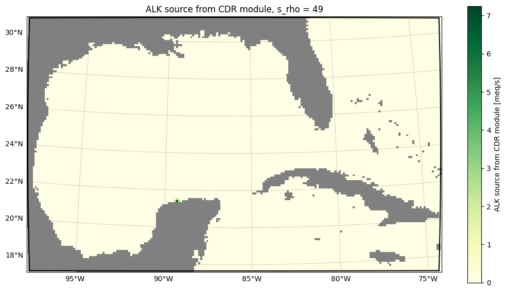
In this experiment, an alkalinity source has been added into the Gulf of Mexico off the coast of the Yucatán Peninsula. This can be visualized by plotting the uppermost layer of ALK_source, a variable from the C-Star output. For more details on visualizing ROMS output fields, see this page.
[5]:
roms_output.plot("ALK_source", s=-1, time=7)
[########################################] | 100% Completed | 101.07 ms
In the next figure, we plot the time series of the total alkalinity source flux.
[6]:
import matplotlib.pyplot as plt
[7]:
def plot_alk_flux_series(ds):
    fig, ax = plt.subplots(figsize=(10, 5))
    ax.plot(ds.time, ds.ALK_source.sum(dim=["eta_rho", "xi_rho", "s_rho"]))
    ax.set(title="Total alkalinity source flux", xlabel="time", ylabel=ds.ALK_source.attrs["units"])
    ax.grid()
[8]:
fig = plot_alk_flux_series(roms_output.ds)
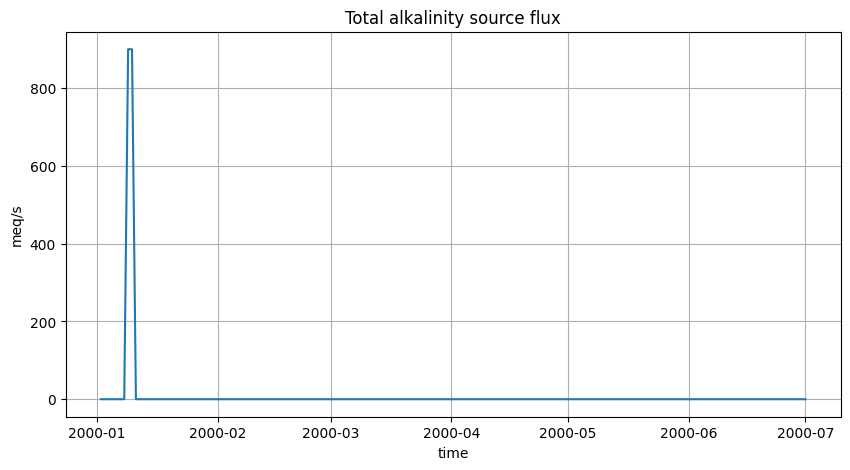
The figure indicates that the release has taken place over a short period in early January 2000.
CO₂ uptake and CDR uptake efficiency#
CDR metrics estimate how much extra CO₂ the ocean takes up because of the intervention, and how efficient that uptake is. The CO₂ uptake is reported as mass in tonnes of CO₂; the efficiency is a dimensionless ratio of moles of DIC transfered from the atmosphere to the ocean per moles of added alkalinity. The same physical story is expressed in two parallel ways (see also here).
Flux-based CO₂ uptake. The first method uses the difference between the air–sea CO₂ flux in the intervention run and in a counter-factual (e.g. alternative CO₂) run. That difference is integrated over the model sea surface and accumulated in time. The implied change in ocean carbon is converted to tonnes of CO₂ using the molar mass of CO₂.
Inventory-based CO₂ uptake. The second method uses the difference in dissolved inorganic carbon between the same two simulations, after accounting for layer thickness and cell geometry so the field represents an inventory per column or per volume element. That difference is integrated over the model domain at each time. Again the result is expressed as tonnes of CO₂ using the same mass conversion.
CDR uptake efficiency. Each uptake construction is normalised by the cumulative source term from the intervention—the added alkalinity (written below as alkalinity source). That yields two efficiency curves over time.
Efficiency from CO₂ flux differences: \begin{equation} \eta_\text{flux}(t_f) = \frac{ \displaystyle \int_{t_0}^{t_f} \int \big( \Phi_\text{intervention} - \Phi_\text{baseline} \big) \, dA \, dt }{ \displaystyle \int_{t_0}^{t_f} \int \text{ALK}_\text{source} \, dV \, dt } \end{equation}
Efficiency from DIC differences: \begin{equation} \eta_\text{DIC}(t_f) = \frac{ \displaystyle \int \big( \text{DIC}_\text{intervention} - \text{DIC}_\text{baseline} \big) \, dV }{ \displaystyle \int_{t_0}^{t_f} \int \text{ALK}_\text{source} \, dV \, dt } \end{equation}
Symbol |
Meaning |
Units |
|---|---|---|
\(t_0\), \(t_f\) |
Start and end times |
s |
\(\Phi_\text{intervention}\), \(\Phi_\mathrm{baseline}\) |
Air–sea CO₂ flux, intervention vs baseline |
mmol/m²/s |
\(\text{DIC}_\text{intervention}\), \(\text{DIC}_\text{baseline}\) |
DIC fields for the two runs evaluated at \(t_f\) |
mmol/m³ |
\(\text{ALK}_\text{source}\) |
Added alkalinity from the intervention |
meq/s |
\(dA\), \(dV\) |
Surface area and volume elements |
m², m³ |
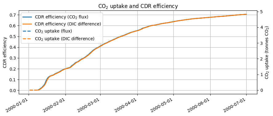
Together, the two methods give two estimates of CO₂ uptake (tonnes CO₂) and two estimates of CDR uptake efficiency; comparing them checks consistency between the flux and inventory views of the same CDR signal. We can perform a CDR analysis, including computing the CDR uptake efficiency and CO\(_2\) uptake in both ways, by calling the method .cdr_metrics(). This method will automatically compute the required diagnostics (if not already present), save them in the attribute .ds_cdr, and produce a plot of the uptake efficiency over time.
[ ]:
roms_output.cdr_metrics()
2026-04-23 12:20:47 - INFO - Max absolute difference between flux-based and DIC-based uptake efficiency: 1.375e-02
A note on discrete integrals, and differences between methods:
Because the numerical model outputs data at discrete intervals, the analytical continuous integrals must be evaluated using finite summations, which can cause discrepancies between the flux-based and DIC inventory based methods.
Flux in the above equations represents the time-averaged gas flux output across the interval \((t_{i-1}, t_i]\), where DIC represents the instantaneous, 3D dissolved inorganic carbon concentrations at the final evaluation time-step \(t_f\). Because the flux-based method involves time averaging from \(t_{i-1}\) to \(t_i\), it lags the DIC inventory method by half a time-step.
CDR-relevant metrics#
After running .cdr_metrics(), a new attribute ds_cdr is created, containing all CDR-relevant outputs.
[10]:
roms_output.ds_cdr
[10]:
<xarray.Dataset> Size: 4GB
Dimensions:                                (time: 182, eta_rho: 130,
                                            xi_rho: 210, s_rho: 50)
Coordinates:
  * time                                   (time) datetime64[ns] 1kB 2000-01-...
    lat_rho                                (eta_rho, xi_rho) float64 218kB 17...
    lon_rho                                (eta_rho, xi_rho) float64 218kB 26...
Dimensions without coordinates: eta_rho, xi_rho, s_rho
Data variables:
    FG_CO2                                 (time, eta_rho, xi_rho) float64 40MB dask.array<chunksize=(1, 130, 210), meta=np.ndarray>
    FG_ALT_CO2                             (time, eta_rho, xi_rho) float64 40MB dask.array<chunksize=(1, 130, 210), meta=np.ndarray>
    hDIC                                   (time, s_rho, eta_rho, xi_rho) float64 2GB dask.array<chunksize=(1, 50, 130, 210), meta=np.ndarray>
    hDIC_ALT_CO2                           (time, s_rho, eta_rho, xi_rho) float64 2GB dask.array<chunksize=(1, 50, 130, 210), meta=np.ndarray>
    area                                   (eta_rho, xi_rho) float64 218kB 1....
    window_length                          (time) float64 1kB dask.array<chunksize=(1,), meta=np.ndarray>
    cdr_efficiency_from_flux               (time) float64 1kB nan nan ... 0.705
    cdr_efficiency_from_DIC_difference     (time) float64 1kB nan nan ... 0.7045
    cdr_carbon_uptake_from_flux            (time) float64 1kB 0.0 0.0 ... 4.825
cdr_carbon_uptake_from_DIC_difference (time) float64 1kB 0.0 0.0 ... 4.822- time: 182
- eta_rho: 130
- xi_rho: 210
- s_rho: 50
- time(time)datetime64[ns]2000-01-02 ... 2000-07-01
array(['2000-01-02T00:00:00.000000000', '2000-01-03T00:00:00.000000000', '2000-01-04T00:00:00.000000000', '2000-01-05T00:00:00.000000000', '2000-01-06T00:00:00.000000000', '2000-01-07T00:00:00.000000000', '2000-01-08T00:00:00.000000000', '2000-01-09T00:00:00.000000000', '2000-01-10T00:00:00.000000000', '2000-01-11T00:00:00.000000000', '2000-01-12T00:00:00.000000000', '2000-01-13T00:00:00.000000000', '2000-01-14T00:00:00.000000000', '2000-01-15T00:00:00.000000000', '2000-01-16T00:00:00.000000000', '2000-01-17T00:00:00.000000000', '2000-01-18T00:00:00.000000000', '2000-01-19T00:00:00.000000000', '2000-01-20T00:00:00.000000000', '2000-01-21T00:00:00.000000000', '2000-01-22T00:00:00.000000000', '2000-01-23T00:00:00.000000000', '2000-01-24T00:00:00.000000000', '2000-01-25T00:00:00.000000000', '2000-01-26T00:00:00.000000000', '2000-01-27T00:00:00.000000000', '2000-01-28T00:00:00.000000000', '2000-01-29T00:00:00.000000000', '2000-01-30T00:00:00.000000000', '2000-01-31T00:00:00.000000000', '2000-02-01T00:00:00.000000000', '2000-02-02T00:00:00.000000000', '2000-02-03T00:00:00.000000000', '2000-02-04T00:00:00.000000000', '2000-02-05T00:00:00.000000000', '2000-02-06T00:00:00.000000000', '2000-02-07T00:00:00.000000000', '2000-02-08T00:00:00.000000000', '2000-02-09T00:00:00.000000000', '2000-02-10T00:00:00.000000000', '2000-02-11T00:00:00.000000000', '2000-02-12T00:00:00.000000000', '2000-02-13T00:00:00.000000000', '2000-02-14T00:00:00.000000000', '2000-02-15T00:00:00.000000000', '2000-02-16T00:00:00.000000000', '2000-02-17T00:00:00.000000000', '2000-02-18T00:00:00.000000000', '2000-02-19T00:00:00.000000000', '2000-02-20T00:00:00.000000000', '2000-02-21T00:00:00.000000000', '2000-02-22T00:00:00.000000000', '2000-02-23T00:00:00.000000000', '2000-02-24T00:00:00.000000000', '2000-02-25T00:00:00.000000000', '2000-02-26T00:00:00.000000000', '2000-02-27T00:00:00.000000000', '2000-02-28T00:00:00.000000000', '2000-02-29T00:00:00.000000000', '2000-03-01T00:00:00.000000000', '2000-03-02T00:00:00.000000000', '2000-03-03T00:00:00.000000000', '2000-03-04T00:00:00.000000000', '2000-03-05T00:00:00.000000000', '2000-03-06T00:00:00.000000000', '2000-03-07T00:00:00.000000000', '2000-03-08T00:00:00.000000000', '2000-03-09T00:00:00.000000000', '2000-03-10T00:00:00.000000000', '2000-03-11T00:00:00.000000000', '2000-03-12T00:00:00.000000000', '2000-03-13T00:00:00.000000000', '2000-03-14T00:00:00.000000000', '2000-03-15T00:00:00.000000000', '2000-03-16T00:00:00.000000000', '2000-03-17T00:00:00.000000000', '2000-03-18T00:00:00.000000000', '2000-03-19T00:00:00.000000000', '2000-03-20T00:00:00.000000000', '2000-03-21T00:00:00.000000000', '2000-03-22T00:00:00.000000000', '2000-03-23T00:00:00.000000000', '2000-03-24T00:00:00.000000000', '2000-03-25T00:00:00.000000000', '2000-03-26T00:00:00.000000000', '2000-03-27T00:00:00.000000000', '2000-03-28T00:00:00.000000000', '2000-03-29T00:00:00.000000000', '2000-03-30T00:00:00.000000000', '2000-03-31T00:00:00.000000000', '2000-04-01T00:00:00.000000000', '2000-04-02T00:00:00.000000000', '2000-04-03T00:00:00.000000000', '2000-04-04T00:00:00.000000000', '2000-04-05T00:00:00.000000000', '2000-04-06T00:00:00.000000000', '2000-04-07T00:00:00.000000000', '2000-04-08T00:00:00.000000000', '2000-04-09T00:00:00.000000000', '2000-04-10T00:00:00.000000000', '2000-04-11T00:00:00.000000000', '2000-04-12T00:00:00.000000000', '2000-04-13T00:00:00.000000000', '2000-04-14T00:00:00.000000000', '2000-04-15T00:00:00.000000000', '2000-04-16T00:00:00.000000000', '2000-04-17T00:00:00.000000000', '2000-04-18T00:00:00.000000000', '2000-04-19T00:00:00.000000000', '2000-04-20T00:00:00.000000000', '2000-04-21T00:00:00.000000000', '2000-04-22T00:00:00.000000000', '2000-04-23T00:00:00.000000000', '2000-04-24T00:00:00.000000000', '2000-04-25T00:00:00.000000000', '2000-04-26T00:00:00.000000000', '2000-04-27T00:00:00.000000000', '2000-04-28T00:00:00.000000000', '2000-04-29T00:00:00.000000000', '2000-04-30T00:00:00.000000000', '2000-05-01T00:00:00.000000000', '2000-05-02T00:00:00.000000000', '2000-05-03T00:00:00.000000000', '2000-05-04T00:00:00.000000000', '2000-05-05T00:00:00.000000000', '2000-05-06T00:00:00.000000000', '2000-05-07T00:00:00.000000000', '2000-05-08T00:00:00.000000000', '2000-05-09T00:00:00.000000000', '2000-05-10T00:00:00.000000000', '2000-05-11T00:00:00.000000000', '2000-05-12T00:00:00.000000000', '2000-05-13T00:00:00.000000000', '2000-05-14T00:00:00.000000000', '2000-05-15T00:00:00.000000000', '2000-05-16T00:00:00.000000000', '2000-05-17T00:00:00.000000000', '2000-05-18T00:00:00.000000000', '2000-05-19T00:00:00.000000000', '2000-05-20T00:00:00.000000000', '2000-05-21T00:00:00.000000000', '2000-05-22T00:00:00.000000000', '2000-05-23T00:00:00.000000000', '2000-05-24T00:00:00.000000000', '2000-05-25T00:00:00.000000000', '2000-05-26T00:00:00.000000000', '2000-05-27T00:00:00.000000000', '2000-05-28T00:00:00.000000000', '2000-05-29T00:00:00.000000000', '2000-05-30T00:00:00.000000000', '2000-05-31T00:00:00.000000000', '2000-06-01T00:00:00.000000000', '2000-06-02T00:00:00.000000000', '2000-06-03T00:00:00.000000000', '2000-06-04T00:00:00.000000000', '2000-06-05T00:00:00.000000000', '2000-06-06T00:00:00.000000000', '2000-06-07T00:00:00.000000000', '2000-06-08T00:00:00.000000000', '2000-06-09T00:00:00.000000000', '2000-06-10T00:00:00.000000000', '2000-06-11T00:00:00.000000000', '2000-06-12T00:00:00.000000000', '2000-06-13T00:00:00.000000000', '2000-06-14T00:00:00.000000000', '2000-06-15T00:00:00.000000000', '2000-06-16T00:00:00.000000000', '2000-06-17T00:00:00.000000000', '2000-06-18T00:00:00.000000000', '2000-06-19T00:00:00.000000000', '2000-06-20T00:00:00.000000000', '2000-06-21T00:00:00.000000000', '2000-06-22T00:00:00.000000000', '2000-06-23T00:00:00.000000000', '2000-06-24T00:00:00.000000000', '2000-06-25T00:00:00.000000000', '2000-06-26T00:00:00.000000000', '2000-06-27T00:00:00.000000000', '2000-06-28T00:00:00.000000000', '2000-06-29T00:00:00.000000000', '2000-06-30T00:00:00.000000000', '2000-07-01T00:00:00.000000000'], dtype='datetime64[ns]') - lat_rho(eta_rho, xi_rho)float6417.08 17.09 17.1 ... 30.92 30.91
- long_name :
- latitude of rho-points
- units :
- degrees North
array([[17.07965766, 17.08870267, 17.09766223, ..., 17.09766223, 17.08870267, 17.07965766], [17.1864053 , 17.19545755, 17.2044243 , ..., 17.2044243 , 17.19545755, 17.1864053 ], [17.29317643, 17.30223593, 17.31120986, ..., 17.31120986, 17.30223593, 17.29317643], ..., [30.69778519, 30.70784508, 30.7178105 , ..., 30.7178105 , 30.70784508, 30.69778519], [30.80446516, 30.81453396, 30.82450821, ..., 30.82450821, 30.81453396, 30.80446516], [30.91112014, 30.92119788, 30.93118098, ..., 30.93118098, 30.92119788, 30.91112014]], shape=(130, 210)) - lon_rho(eta_rho, xi_rho)float64262.3 262.4 262.5 ... 287.0 287.1
- long_name :
- longitude of rho-points
- units :
- degrees East
array([[262.28326465, 262.39493133, 262.50661093, ..., 285.49338907,
        285.60506867, 285.71673535],
       [262.27375111, 262.38550674, 262.49727537, ..., 285.50272463,
        285.61449326, 285.72624889],
       [262.26422446, 262.37606917, 262.48792693, ..., 285.51207307,
        285.62393083, 285.73577554],
       ...,
       [260.94698334, 261.07107419, 261.19518823, ..., 286.80481177,
        286.92892581, 287.05301666],
       [260.93521741, 261.05941698, 261.18363985, ..., 286.81636015,
        286.94058302, 287.06478259],
       [260.92342798, 261.04773647, 261.17206838, ..., 286.82793162,
        286.95226353, 287.07657202]], shape=(130, 210))
- FG_CO2(time, eta_rho, xi_rho)float64dask.array<chunksize=(1, 130, 210), meta=np.ndarray>
- long_name :
- DIC Surface Gas Flux
- units :
- mmol/m^2/s
Array Chunk Bytes 37.91 MiB 213.28 kiB Shape (182, 130, 210) (1, 130, 210) Dask graph 182 chunks in 3 graph layers Data type float64 numpy.ndarray - FG_ALT_CO2(time, eta_rho, xi_rho)float64dask.array<chunksize=(1, 130, 210), meta=np.ndarray>
- long_name :
- DIC Surface Gas Flux, Alternative CO2
- units :
- mmol/m^2/s
Array Chunk Bytes 37.91 MiB 213.28 kiB Shape (182, 130, 210) (1, 130, 210) Dask graph 182 chunks in 3 graph layers Data type float64 numpy.ndarray - hDIC(time, s_rho, eta_rho, xi_rho)float64dask.array<chunksize=(1, 50, 130, 210), meta=np.ndarray>
- long_name :
- thickness-weighted Dissolved Inorganic Carbon
- units :
- meters mmol/m^3
Array Chunk Bytes 1.85 GiB 10.41 MiB Shape (182, 50, 130, 210) (1, 50, 130, 210) Dask graph 182 chunks in 3 graph layers Data type float64 numpy.ndarray - hDIC_ALT_CO2(time, s_rho, eta_rho, xi_rho)float64dask.array<chunksize=(1, 50, 130, 210), meta=np.ndarray>
- long_name :
- thickness-weighted Dissolved Inorganic Carbon, Alternative CO2
- units :
- meters mmol/m^3
Array Chunk Bytes 1.85 GiB 10.41 MiB Shape (182, 50, 130, 210) (1, 50, 130, 210) Dask graph 182 chunks in 3 graph layers Data type float64 numpy.ndarray - area(eta_rho, xi_rho)float641.419e+08 1.419e+08 ... 1.419e+08
- long_name :
- Grid cell area
- units :
- m^2
array([[1.41927725e+08, 1.41927725e+08, 1.41927725e+08, ..., 1.41927725e+08, 1.41927725e+08, 1.41927725e+08], [1.41959795e+08, 1.41959795e+08, 1.41959795e+08, ..., 1.41959795e+08, 1.41959795e+08, 1.41959795e+08], [1.42022965e+08, 1.42022965e+08, 1.42022965e+08, ..., 1.42022965e+08, 1.42022965e+08, 1.42022965e+08], ..., [1.42022965e+08, 1.42022965e+08, 1.42022965e+08, ..., 1.42022965e+08, 1.42022965e+08, 1.42022965e+08], [1.41959795e+08, 1.41959795e+08, 1.41959795e+08, ..., 1.41959795e+08, 1.41959795e+08, 1.41959795e+08], [1.41927725e+08, 1.41927725e+08, 1.41927725e+08, ..., 1.41927725e+08, 1.41927725e+08, 1.41927725e+08]], shape=(130, 210)) - window_length(time)float64dask.array<chunksize=(1,), meta=np.ndarray>
- long_name :
- Duration of each averaging window
- units :
- s
Array Chunk Bytes 1.42 kiB 8 B Shape (182,) (1,) Dask graph 182 chunks in 7 graph layers Data type float64 numpy.ndarray - cdr_efficiency_from_flux(time)float64nan nan nan ... 0.7035 0.7043 0.705
- long_name :
- CDR uptake efficiency (from flux differences)
- units :
- nondimensional
- description :
- Carbon Dioxide Removal efficiency computed using area-integrated CO2 flux differences
array([ nan, nan, nan, nan, nan, nan, nan, 0.00352773, 0.00769334, 0.01537455, 0.02428025, 0.0352017 , 0.04700555, 0.06747976, 0.09472376, 0.11233898, 0.12435776, 0.13168928, 0.13466993, 0.13855525, 0.14377533, 0.15104856, 0.1563381 , 0.16149247, 0.1667724 , 0.1715628 , 0.17937107, 0.1866191 , 0.19104804, 0.19643639, 0.19932857, 0.20235916, 0.20610844, 0.20932456, 0.21468369, 0.22619296, 0.23371094, 0.24309953, 0.25248173, 0.26028267, 0.26355729, 0.27031728, 0.27941941, 0.28713768, 0.29216281, 0.29739223, 0.30529974, 0.312476 , 0.32129395, 0.32989682, 0.3396997 , 0.35029992, 0.3607551 , 0.37024045, 0.37783029, 0.38547304, 0.39203915, 0.39662096, 0.40389306, 0.41001443, 0.41678714, 0.42340817, 0.42948809, 0.43410147, 0.43858193, 0.44403248, 0.45022117, 0.45553424, 0.46045843, 0.46541554, 0.47020147, 0.47511887, 0.4805188 , 0.48597858, 0.49096205, 0.4956597 , 0.49889566, 0.50306955, 0.50735121, 0.51096432, 0.51565928, 0.52072434, 0.52507779, 0.52964413, 0.53453956, 0.53836808, 0.54146478, 0.54436808, 0.54795609, 0.55075637, 0.55354198, 0.55724825, 0.56148456, 0.56625196, 0.57331876, 0.57740005, 0.58108331, 0.58419487, 0.58723731, 0.59173012, 0.59555043, 0.59825449, 0.6010791 , 0.60292248, 0.60405801, 0.60553418, 0.60799568, 0.61030399, 0.61291308, 0.61557384, 0.61791122, 0.61968439, 0.62155471, 0.62331343, 0.62506004, 0.62626934, 0.62818642, 0.63048342, 0.63259224, 0.63434816, 0.63635571, 0.63865499, 0.64088295, 0.64280101, 0.64466381, 0.64633047, 0.64790299, 0.64959933, 0.65104364, 0.65257192, 0.6540106 , 0.65537789, 0.65661733, 0.65819997, 0.65975381, 0.66155947, 0.66283453, 0.66375733, 0.66499772, 0.66597938, 0.66689366, 0.66774988, 0.66863776, 0.66978134, 0.6705346 , 0.67150096, 0.6726483 , 0.67373736, 0.67451561, 0.67549447, 0.67609306, 0.67704561, 0.67807112, 0.67905787, 0.68023696, 0.68137623, 0.68230832, 0.68306854, 0.68355924, 0.68444954, 0.685128 , 0.68593106, 0.68689424, 0.68800248, 0.68931254, 0.69033233, 0.69118183, 0.6921384 , 0.6932609 , 0.69458233, 0.69576017, 0.69666555, 0.69767668, 0.69863188, 0.69948905, 0.7002746 , 0.70111486, 0.70200928, 0.70285372, 0.70348485, 0.70429405, 0.7050147 ]) - cdr_efficiency_from_DIC_difference(time)float64nan nan nan ... 0.7038 0.7045
- long_name :
- CDR uptake efficiency (from DIC differences)
- units :
- nondimensional
- description :
- Carbon Dioxide Removal efficiency computed using volume-integrated DIC differences
array([ nan, nan, nan, nan, nan, nan, nan, 0.00123677, 0.00466054, 0.01175855, 0.01964947, 0.03032238, 0.04115548, 0.05620005, 0.08097641, 0.1042102 , 0.11865996, 0.12887325, 0.13355418, 0.13661414, 0.14138894, 0.14811533, 0.15429169, 0.15793378, 0.16481668, 0.16893075, 0.1756266 , 0.18357174, 0.18892452, 0.19420981, 0.19818707, 0.20090362, 0.20440272, 0.20777847, 0.21106866, 0.22065466, 0.22985652, 0.23852439, 0.24763328, 0.25682094, 0.26211623, 0.26719781, 0.27555156, 0.2841777 , 0.2897502 , 0.29504937, 0.30169743, 0.3096187 , 0.31730202, 0.3256761 , 0.33507954, 0.34485525, 0.35627398, 0.36623435, 0.37440939, 0.3824465 , 0.38898257, 0.39468224, 0.40045845, 0.4076699 , 0.41354916, 0.42084067, 0.4267707 , 0.43211297, 0.43683116, 0.44150863, 0.44772709, 0.45324122, 0.45808641, 0.46337077, 0.46810442, 0.4728178 , 0.47828524, 0.48387746, 0.48878288, 0.49371827, 0.49720166, 0.50132096, 0.50538647, 0.50948359, 0.51356996, 0.51841994, 0.52305264, 0.52769705, 0.53255828, 0.53699021, 0.54010976, 0.54317408, 0.54643 , 0.54945414, 0.55216286, 0.5556243 , 0.55973014, 0.56410844, 0.56893389, 0.57585507, 0.57945955, 0.58302681, 0.58581412, 0.58947972, 0.59411406, 0.5970534 , 0.59978647, 0.60220253, 0.60354215, 0.60494945, 0.60692615, 0.60929998, 0.61183407, 0.61451216, 0.6169044 , 0.61899169, 0.62080806, 0.62262164, 0.62424654, 0.62567109, 0.62733438, 0.6295094 , 0.63174816, 0.63360968, 0.63538921, 0.63762538, 0.63990315, 0.64193695, 0.64389796, 0.64558391, 0.64720039, 0.64888523, 0.65034429, 0.65193969, 0.65335621, 0.65477552, 0.65601027, 0.65739495, 0.65898264, 0.66065647, 0.66232569, 0.66340911, 0.66443994, 0.66555255, 0.66644773, 0.66732655, 0.66825091, 0.66928789, 0.67016286, 0.67103717, 0.6721832 , 0.6732626 , 0.67404025, 0.67503305, 0.67571534, 0.67654983, 0.67759176, 0.67851324, 0.67972476, 0.68092128, 0.68191634, 0.68275198, 0.68332517, 0.6840492 , 0.68478184, 0.68548994, 0.68643337, 0.68741961, 0.68872222, 0.68993022, 0.69080148, 0.69172959, 0.69272381, 0.69394197, 0.69521851, 0.69615051, 0.6971333 , 0.69808794, 0.69901856, 0.69981963, 0.70054888, 0.70139584, 0.70230743, 0.70305795, 0.70377672, 0.70453142]) - cdr_carbon_uptake_from_flux(time)float640.0 0.0 0.0 ... 4.815 4.82 4.825
- long_name :
- CDR carbon uptake (cumulative flux differences)
- units :
- tonnes CO2
- description :
- Time-cumulative CO2 uptake mass from area-integrated CO2 flux differences (scenario minus reference), converted from native DIC carbon units using FG_CO2 units metadata when present (otherwise mmol is assumed). Same quantity as the numerator of flux-based efficiency before dividing by the source, expressed as tonnes CO2.
array([0. , 0. , 0. , 0. , 0. , 0. , 0. , 0.01207265, 0.05265659, 0.10523011, 0.1661846 , 0.24093575, 0.32172641, 0.46186083, 0.64833063, 0.76889688, 0.85115863, 0.90133872, 0.92173963, 0.9483324 , 0.98406096, 1.03384206, 1.07004603, 1.10532477, 1.14146291, 1.1742505 , 1.22769364, 1.27730237, 1.30761591, 1.34449614, 1.36429148, 1.38503416, 1.41069583, 1.43270839, 1.46938857, 1.54816306, 1.5996194 , 1.663879 , 1.72809483, 1.78148784, 1.80390077, 1.85016909, 1.91246807, 1.96529524, 1.99968945, 2.03548182, 2.08960427, 2.13872176, 2.19907562, 2.2579574 , 2.3250526 , 2.39760512, 2.46916492, 2.53408676, 2.58603491, 2.63834522, 2.68328654, 2.71464648, 2.76441986, 2.80631717, 2.85267256, 2.89798977, 2.93960343, 2.97117936, 3.00184562, 3.03915154, 3.0815096 , 3.1178746 , 3.15157791, 3.1855065 , 3.21826348, 3.25192033, 3.28887981, 3.32624891, 3.36035796, 3.3925107 , 3.41465905, 3.44322691, 3.47253246, 3.49726214, 3.52939656, 3.56406399, 3.59386094, 3.62511494, 3.65862138, 3.68482545, 3.70602058, 3.72589204, 3.75044994, 3.76961626, 3.78868218, 3.81404954, 3.84304471, 3.87567482, 3.92404313, 3.95197722, 3.97718707, 3.99848395, 4.01930774, 4.05005844, 4.07620633, 4.09471411, 4.11404698, 4.12666382, 4.13443589, 4.14453944, 4.16138701, 4.1771861 , 4.19504385, 4.21325529, 4.2292533 , 4.24138966, 4.25419094, 4.26622835, 4.27818292, 4.28645993, 4.29958124, 4.31530293, 4.32973659, 4.3417549 , 4.35549545, 4.37123272, 4.38648179, 4.39960984, 4.41235968, 4.42376699, 4.43453005, 4.4461405 , 4.45602601, 4.46648624, 4.4763332 , 4.48569152, 4.49417479, 4.50500706, 4.51564221, 4.52800093, 4.53672796, 4.54304404, 4.55153379, 4.55825271, 4.56451047, 4.57037077, 4.5764478 , 4.584275 , 4.58943064, 4.59604484, 4.60389768, 4.61135167, 4.61667839, 4.62337815, 4.62747516, 4.63399479, 4.64101386, 4.64776758, 4.65583782, 4.66363547, 4.67001505, 4.67521833, 4.67857692, 4.68467049, 4.6893142 , 4.69481072, 4.7014031 , 4.70898837, 4.71795499, 4.72493489, 4.73074927, 4.73729642, 4.74497933, 4.75402374, 4.76208542, 4.76828222, 4.7752028 , 4.7817406 , 4.78760746, 4.79298411, 4.79873521, 4.80485701, 4.81063673, 4.81495644, 4.82049498, 4.82542742]) - cdr_carbon_uptake_from_DIC_difference(time)float640.0 0.0 0.0 ... 4.812 4.817 4.822
- long_name :
- CDR carbon uptake (from DIC differences)
- units :
- tonnes CO2
- description :
- CO2-equivalent mass from the volume-integrated DIC difference (scenario minus reference), converted from native DIC carbon units using hDIC units metadata when present (otherwise mmol is assumed). Same quantity as the numerator of DIC-based efficiency before dividing by the source, expressed as tonnes CO2.
array([0.00000000e+00, 0.00000000e+00, 0.00000000e+00, 0.00000000e+00,
       0.00000000e+00, 0.00000000e+00, 0.00000000e+00, 4.23248338e-03,
       3.18987303e-02, 8.04806419e-02, 1.34489538e-01, 2.07539547e-01,
       2.81685996e-01, 3.84657612e-01, 5.54237824e-01, 7.13259937e-01,
       8.12160410e-01, 8.82064622e-01, 9.14102913e-01, 9.35046607e-01,
       9.67727412e-01, 1.01376579e+00, 1.05603947e+00, 1.08096754e+00,
       1.12807711e+00, 1.15623560e+00, 1.20206486e+00, 1.25644488e+00,
       1.29308162e+00, 1.32925644e+00, 1.35647855e+00, 1.37507180e+00,
       1.39902118e+00, 1.42212626e+00, 1.44464575e+00, 1.51025651e+00,
       1.57323807e+00, 1.63256474e+00, 1.69490996e+00, 1.75779425e+00,
       1.79403758e+00, 1.82881812e+00, 1.88599478e+00, 1.94503588e+00,
       1.98317650e+00, 2.01944631e+00, 2.06494850e+00, 2.11916514e+00,
       2.17175314e+00, 2.22906898e+00, 2.29343020e+00, 2.36033939e+00,
       2.43849420e+00, 2.50666731e+00, 2.56262082e+00, 2.61763031e+00,
       2.66236598e+00, 2.70137704e+00, 2.74091191e+00, 2.79027018e+00,
       2.83051043e+00, 2.88041668e+00, 2.92100443e+00, 2.95756925e+00,
       2.98986256e+00, 3.02187724e+00, 3.06443908e+00, 3.10218019e+00,
       3.13534278e+00, 3.17151123e+00, 3.20391034e+00, 3.23617080e+00,
       3.27359231e+00, 3.31186792e+00, 3.34544274e+00, 3.37922268e+00,
       3.40306458e+00, 3.43125881e+00, 3.45908498e+00, 3.48712740e+00,
...
       4.13090516e+00, 4.14053729e+00, 4.15406670e+00, 4.17031424e+00,
       4.18765863e+00, 4.20598863e+00, 4.22236216e+00, 4.23664854e+00,
       4.24908051e+00, 4.26149350e+00, 4.27261496e+00, 4.28236520e+00,
       4.29374951e+00, 4.30863631e+00, 4.32395932e+00, 4.33670041e+00,
       4.34888026e+00, 4.36418560e+00, 4.37977562e+00, 4.39369589e+00,
       4.40711789e+00, 4.41865722e+00, 4.42972113e+00, 4.44125291e+00,
       4.45123936e+00, 4.46215898e+00, 4.47185423e+00, 4.48156862e+00,
       4.49001977e+00, 4.49949716e+00, 4.51036399e+00, 4.52182040e+00,
       4.53324528e+00, 4.54066067e+00, 4.54771615e+00, 4.55533128e+00,
       4.56145828e+00, 4.56747332e+00, 4.57380007e+00, 4.58089759e+00,
       4.58688629e+00, 4.59287039e+00, 4.60071437e+00, 4.60810226e+00,
       4.61342480e+00, 4.62022000e+00, 4.62488986e+00, 4.63060148e+00,
       4.63773289e+00, 4.64403994e+00, 4.65233204e+00, 4.66052157e+00,
       4.66733219e+00, 4.67305166e+00, 4.67697482e+00, 4.68193039e+00,
       4.68694496e+00, 4.69179149e+00, 4.69824873e+00, 4.70499895e+00,
       4.71391458e+00, 4.72218270e+00, 4.72814597e+00, 4.73449837e+00,
       4.74130322e+00, 4.74964084e+00, 4.75837802e+00, 4.76475702e+00,
       4.77148370e+00, 4.77801767e+00, 4.78438725e+00, 4.78987009e+00,
       4.79486139e+00, 4.80065835e+00, 4.80689772e+00, 4.81203459e+00,
       4.81695415e+00, 4.82211965e+00])
- timePandasIndex
PandasIndex(DatetimeIndex(['2000-01-02', '2000-01-03', '2000-01-04', '2000-01-05',
               '2000-01-06', '2000-01-07', '2000-01-08', '2000-01-09',
               '2000-01-10', '2000-01-11',
               ...
               '2000-06-22', '2000-06-23', '2000-06-24', '2000-06-25',
               '2000-06-26', '2000-06-27', '2000-06-28', '2000-06-29',
               '2000-06-30', '2000-07-01'],
              dtype='datetime64[ns]', name='time', length=182, freq=None))
We can save the CDR-relevant outputs (stored in .ds_cdr) to a NetCDF file using xarray’s .to_netcdf() method.
[11]:
cdr_filepath = "/pscratch/sd/u/uheede/output/cdr_metrics.nc"
[12]:
roms_output.ds_cdr.to_netcdf(cdr_filepath)
Ensembles of CDR efficiency curves#
Let’s now look at ensembles. For this we have run a second CDR experiment. Let’s open its output!
[13]:
another_roms_output = ROMSOutput(
    grid=grid,
    path=[
        "/global/cfs/projectdirs/m4746/Datasets/ROMSOutput/gom12km/atlas_cdr2_cstar.nc"
    ],
    use_dask=True,
)
The release location is the same as in the first CDR experiment.
[14]:
another_roms_output.plot("ALK_source", s=-1, time=7)
[########################################] | 100% Completed | 101.21 ms
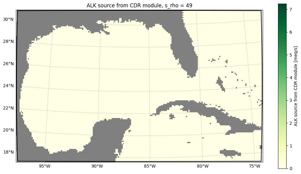
However, plotting the total alkalinity source flux indicates that the release occurred over a short period in early April 2000, whereas in the first experiment it took place in early January 2000.
[15]:
fig = plot_alk_flux_series(another_roms_output.ds)
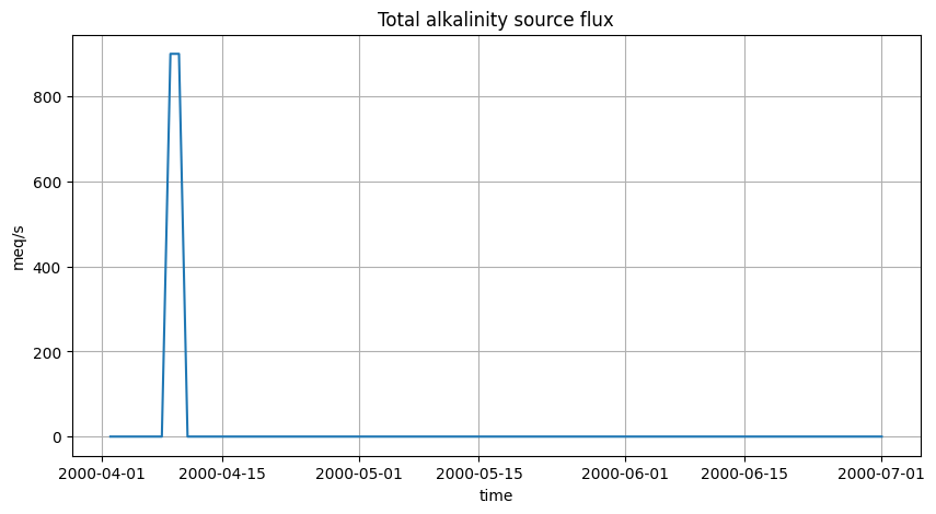
Note also that the second experiment only ran for three months, while the first ran for six months.
[16]:
another_roms_output.cdr_metrics()
2026-04-23 12:22:52 - INFO - Max absolute difference between flux-based and DIC-based uptake efficiency: 1.088e-02
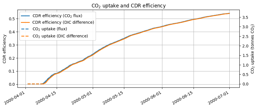
We can now construct a small ensemble consisting of two members: our two experiments. Note that ensemble members do not need to share the same start or end dates.
[17]:
from roms_tools import Ensemble
The members variable is a dictionary whose values can be either:
file paths (strings) pointing to the CDR metrics, or
xarray.Datasetobjects containing the metrics directly.
Let’s use a mix of both!
[18]:
ensemble = Ensemble(
    members={
        "January_release": cdr_filepath,
        "April_release": another_roms_output.ds_cdr
    }
)
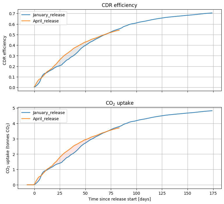
The .ds attribute contains an xarray.Dataset that aggregates all releases, aligns them relative to the release start date, and computes the ensemble mean and standard deviation for both efficiency and CO\(_2\) uptake.
[19]:
ensemble.ds
[19]:
<xarray.Dataset> Size: 13kB
Dimensions:                     (time: 182)
Coordinates:
  * time                        (time) timedelta64[s] 1kB -7 days ... 174 days
Data variables:
    January_release             (time) float64 1kB nan nan nan ... 0.7043 0.705
    April_release               (time) float64 1kB nan nan nan ... nan nan nan
    ensemble_efficiency_mean    (time) float64 1kB nan nan nan ... 0.7043 0.705
    ensemble_efficiency_std     (time) float64 1kB nan nan nan ... 0.0 0.0 0.0
    January_release_co2_uptake  (time) float64 1kB 0.0 0.0 0.0 ... 4.82 4.825
    April_release_co2_uptake    (time) float64 1kB 0.0 0.0 0.0 ... nan nan nan
    ensemble_uptake_mean        (time) float64 1kB 0.0 0.0 0.0 ... 4.82 4.825
ensemble_uptake_std (time) float64 1kB 0.0 0.0 0.0 ... 0.0 0.0 0.0- time: 182
- time(time)timedelta64[s]-7 days -6 days ... 174 days
- long_name :
- time since release start
array([ -604800,  -518400,  -432000,  -345600,  -259200,  -172800,   -86400,
              0,    86400,   172800,   259200,   345600,   432000,   518400,
         604800,   691200,   777600,   864000,   950400,  1036800,  1123200,
        1209600,  1296000,  1382400,  1468800,  1555200,  1641600,  1728000,
        1814400,  1900800,  1987200,  2073600,  2160000,  2246400,  2332800,
        2419200,  2505600,  2592000,  2678400,  2764800,  2851200,  2937600,
        3024000,  3110400,  3196800,  3283200,  3369600,  3456000,  3542400,
        3628800,  3715200,  3801600,  3888000,  3974400,  4060800,  4147200,
        4233600,  4320000,  4406400,  4492800,  4579200,  4665600,  4752000,
        4838400,  4924800,  5011200,  5097600,  5184000,  5270400,  5356800,
        5443200,  5529600,  5616000,  5702400,  5788800,  5875200,  5961600,
        6048000,  6134400,  6220800,  6307200,  6393600,  6480000,  6566400,
        6652800,  6739200,  6825600,  6912000,  6998400,  7084800,  7171200,
        7257600,  7344000,  7430400,  7516800,  7603200,  7689600,  7776000,
        7862400,  7948800,  8035200,  8121600,  8208000,  8294400,  8380800,
        8467200,  8553600,  8640000,  8726400,  8812800,  8899200,  8985600,
        9072000,  9158400,  9244800,  9331200,  9417600,  9504000,  9590400,
        9676800,  9763200,  9849600,  9936000, 10022400, 10108800, 10195200,
       10281600, 10368000, 10454400, 10540800, 10627200, 10713600, 10800000,
       10886400, 10972800, 11059200, 11145600, 11232000, 11318400, 11404800,
       11491200, 11577600, 11664000, 11750400, 11836800, 11923200, 12009600,
       12096000, 12182400, 12268800, 12355200, 12441600, 12528000, 12614400,
       12700800, 12787200, 12873600, 12960000, 13046400, 13132800, 13219200,
       13305600, 13392000, 13478400, 13564800, 13651200, 13737600, 13824000,
       13910400, 13996800, 14083200, 14169600, 14256000, 14342400, 14428800,
       14515200, 14601600, 14688000, 14774400, 14860800, 14947200, 15033600],
      dtype='timedelta64[s]')
- January_release(time)float64nan nan nan ... 0.7035 0.7043 0.705
- long_name :
- CDR uptake efficiency (from flux differences)
- units :
- nondimensional
- description :
- Carbon Dioxide Removal efficiency computed using area-integrated CO2 flux differences
array([ nan, nan, nan, nan, nan, nan, nan, 0.003528, 0.007693, 0.015375, 0.02428 , 0.035202, 0.047006, 0.06748 , 0.094724, 0.112339, 0.124358, 0.131689, 0.13467 , 0.138555, 0.143775, 0.151049, 0.156338, 0.161492, 0.166772, 0.171563, 0.179371, 0.186619, 0.191048, 0.196436, 0.199329, 0.202359, 0.206108, 0.209325, 0.214684, 0.226193, 0.233711, 0.2431 , 0.252482, 0.260283, 0.263557, 0.270317, 0.279419, 0.287138, 0.292163, 0.297392, 0.3053 , 0.312476, 0.321294, 0.329897, 0.3397 , 0.3503 , 0.360755, 0.37024 , 0.37783 , 0.385473, 0.392039, 0.396621, 0.403893, 0.410014, 0.416787, 0.423408, 0.429488, 0.434101, 0.438582, 0.444032, 0.450221, 0.455534, 0.460458, 0.465416, 0.470201, 0.475119, 0.480519, 0.485979, 0.490962, 0.49566 , 0.498896, 0.50307 , 0.507351, 0.510964, 0.515659, 0.520724, 0.525078, 0.529644, 0.53454 , 0.538368, 0.541465, 0.544368, 0.547956, 0.550756, 0.553542, 0.557248, 0.561485, 0.566252, 0.573319, 0.5774 , 0.581083, 0.584195, 0.587237, 0.59173 , 0.59555 , 0.598254, 0.601079, 0.602922, 0.604058, 0.605534, 0.607996, 0.610304, 0.612913, 0.615574, 0.617911, 0.619684, 0.621555, 0.623313, 0.62506 , 0.626269, 0.628186, 0.630483, 0.632592, 0.634348, 0.636356, 0.638655, 0.640883, 0.642801, 0.644664, 0.64633 , 0.647903, 0.649599, 0.651044, 0.652572, 0.654011, 0.655378, 0.656617, 0.6582 , 0.659754, 0.661559, 0.662835, 0.663757, 0.664998, 0.665979, 0.666894, 0.66775 , 0.668638, 0.669781, 0.670535, 0.671501, 0.672648, 0.673737, 0.674516, 0.675494, 0.676093, 0.677046, 0.678071, 0.679058, 0.680237, 0.681376, 0.682308, 0.683069, 0.683559, 0.68445 , 0.685128, 0.685931, 0.686894, 0.688002, 0.689313, 0.690332, 0.691182, 0.692138, 0.693261, 0.694582, 0.69576 , 0.696666, 0.697677, 0.698632, 0.699489, 0.700275, 0.701115, 0.702009, 0.702854, 0.703485, 0.704294, 0.705015]) - April_release(time)float64nan nan nan nan ... nan nan nan nan
- long_name :
- CDR uptake efficiency (from flux differences)
- units :
- nondimensional
- description :
- Carbon Dioxide Removal efficiency computed using area-integrated CO2 flux differences
array([ nan, nan, nan, nan, nan, nan, nan, 0.00676998, 0.02064941, 0.03947279, 0.05420447, 0.06908475, 0.07824617, 0.08241208, 0.08953579, 0.10024155, 0.11095466, 0.12052425, 0.13237953, 0.14421083, 0.15195782, 0.15748828, 0.16403231, 0.17282637, 0.17712805, 0.18686859, 0.19953817, 0.2091211 , 0.21677561, 0.22741454, 0.23939558, 0.25113105, 0.26193187, 0.27153093, 0.28154843, 0.29035054, 0.29954171, 0.30707249, 0.31349777, 0.32055194, 0.32742618, 0.3344551 , 0.34220009, 0.34902481, 0.35747904, 0.36576083, 0.37255186, 0.37794849, 0.38315302, 0.38765613, 0.39288031, 0.3988102 , 0.40454004, 0.40923163, 0.41465732, 0.42048587, 0.42612552, 0.42976378, 0.43286144, 0.43635654, 0.44085197, 0.44565071, 0.45052435, 0.45472348, 0.45782829, 0.46136779, 0.46416136, 0.46722233, 0.47100128, 0.4747407 , 0.47894388, 0.48341535, 0.48760917, 0.49159394, 0.49463948, 0.49753113, 0.5004113 , 0.50403751, 0.50807128, 0.51210103, 0.51515995, 0.51795879, 0.52073572, 0.52353277, 0.52620842, 0.52909885, 0.53180912, 0.53516934, 0.53702319, 0.5385916 , 0.54097839, nan, nan, nan, nan, nan, nan, nan, nan, nan, nan, nan, nan, nan, nan, nan, nan, nan, nan, nan, nan, nan, nan, nan, nan, nan, nan, nan, nan, nan, nan, nan, nan, nan, nan, nan, nan, nan, nan, nan, nan, nan, nan, nan, nan, nan, nan, nan, nan, nan, nan, nan, nan, nan, nan, nan, nan, nan, nan, nan, nan, nan, nan, nan, nan, nan, nan, nan, nan, nan, nan, nan, nan, nan, nan, nan, nan, nan, nan, nan, nan, nan, nan, nan, nan, nan, nan, nan, nan, nan, nan, nan]) - ensemble_efficiency_mean(time)float64nan nan nan ... 0.7035 0.7043 0.705
array([ nan, nan, nan, nan, nan, nan, nan, 0.00514886, 0.01417138, 0.02742367, 0.03924236, 0.05214323, 0.06262586, 0.07494592, 0.09212977, 0.10629026, 0.11765621, 0.12610676, 0.13352473, 0.14138304, 0.14786658, 0.15426842, 0.16018521, 0.16715942, 0.17195023, 0.1792157 , 0.18945462, 0.1978701 , 0.20391182, 0.21192546, 0.21936207, 0.22674511, 0.23402015, 0.24042774, 0.24811606, 0.25827175, 0.26662633, 0.27508601, 0.28298975, 0.2904173 , 0.29549173, 0.30238619, 0.31080975, 0.31808124, 0.32482093, 0.33157653, 0.3389258 , 0.34521225, 0.35222348, 0.35877648, 0.36629001, 0.37455506, 0.38264757, 0.38973604, 0.3962438 , 0.40297945, 0.40908234, 0.41319237, 0.41837725, 0.42318548, 0.42881955, 0.43452944, 0.44000622, 0.44441247, 0.44820511, 0.45270014, 0.45719126, 0.46137829, 0.46572986, 0.47007812, 0.47457267, 0.47926711, 0.48406399, 0.48878626, 0.49280077, 0.49659542, 0.49965348, 0.50355353, 0.50771124, 0.51153267, 0.51540962, 0.51934157, 0.52290676, 0.52658845, 0.53037399, 0.53373347, 0.53663695, 0.53976871, 0.54248964, 0.54467398, 0.54726018, 0.55724825, 0.56148456, 0.56625196, 0.57331876, 0.57740005, 0.58108331, 0.58419487, 0.58723731, 0.59173012, 0.59555043, 0.59825449, 0.6010791 , 0.60292248, 0.60405801, 0.60553418, 0.60799568, 0.61030399, 0.61291308, 0.61557384, 0.61791122, 0.61968439, 0.62155471, 0.62331343, 0.62506004, 0.62626934, 0.62818642, 0.63048342, 0.63259224, 0.63434816, 0.63635571, 0.63865499, 0.64088295, 0.64280101, 0.64466381, 0.64633047, 0.64790299, 0.64959933, 0.65104364, 0.65257192, 0.6540106 , 0.65537789, 0.65661733, 0.65819997, 0.65975381, 0.66155947, 0.66283453, 0.66375733, 0.66499772, 0.66597938, 0.66689366, 0.66774988, 0.66863776, 0.66978134, 0.6705346 , 0.67150096, 0.6726483 , 0.67373736, 0.67451561, 0.67549447, 0.67609306, 0.67704561, 0.67807112, 0.67905787, 0.68023696, 0.68137623, 0.68230832, 0.68306854, 0.68355924, 0.68444954, 0.685128 , 0.68593106, 0.68689424, 0.68800248, 0.68931254, 0.69033233, 0.69118183, 0.6921384 , 0.6932609 , 0.69458233, 0.69576017, 0.69666555, 0.69767668, 0.69863188, 0.69948905, 0.7002746 , 0.70111486, 0.70200928, 0.70285372, 0.70348485, 0.70429405, 0.7050147 ]) - ensemble_efficiency_std(time)float64nan nan nan nan ... 0.0 0.0 0.0 0.0
array([ nan, nan, nan, nan, nan, nan, nan, 0.00162113, 0.00647803, 0.01204912, 0.01496211, 0.01694153, 0.01562031, 0.00746616, 0.00259399, 0.00604872, 0.00670155, 0.00558251, 0.0011452 , 0.00282779, 0.00409124, 0.00321986, 0.0038471 , 0.00566695, 0.00517782, 0.00765289, 0.01008355, 0.011251 , 0.01286379, 0.01548907, 0.0200335 , 0.02438595, 0.02791172, 0.03110318, 0.03343237, 0.03207879, 0.03291538, 0.03198648, 0.03050802, 0.03013464, 0.03193445, 0.03206891, 0.03139034, 0.03094356, 0.03265811, 0.0341843 , 0.03362606, 0.03273624, 0.03092953, 0.02887966, 0.0265903 , 0.02425514, 0.02189247, 0.01949559, 0.01841352, 0.01750642, 0.01704319, 0.01657141, 0.01448419, 0.01317106, 0.01203241, 0.01112127, 0.01051813, 0.010311 , 0.00962318, 0.00866765, 0.0069701 , 0.00584404, 0.00527142, 0.00466258, 0.0043712 , 0.00414824, 0.00354518, 0.00280768, 0.00183871, 0.00093571, 0.00075782, 0.00048398, 0.00036003, 0.00056836, 0.00024967, 0.00138277, 0.00217104, 0.00305568, 0.00416557, 0.00463461, 0.00482783, 0.00459937, 0.00546645, 0.00608238, 0.00628179, 0. , 0. , 0. , 0. , 0. , 0. , 0. , 0. , 0. , 0. , 0. , 0. , 0. , 0. , 0. , 0. , 0. , 0. , 0. , 0. , 0. , 0. , 0. , 0. , 0. , 0. , 0. , 0. , 0. , 0. , 0. , 0. , 0. , 0. , 0. , 0. , 0. , 0. , 0. , 0. , 0. , 0. , 0. , 0. , 0. , 0. , 0. , 0. , 0. , 0. , 0. , 0. , 0. , 0. , 0. , 0. , 0. , 0. , 0. , 0. , 0. , 0. , 0. , 0. , 0. , 0. , 0. , 0. , 0. , 0. , 0. , 0. , 0. , 0. , 0. , 0. , 0. , 0. , 0. , 0. , 0. , 0. , 0. , 0. , 0. , 0. , 0. , 0. , 0. , 0. , 0. ]) - January_release_co2_uptake(time)float640.0 0.0 0.0 ... 4.815 4.82 4.825
- long_name :
- CDR carbon uptake (cumulative flux differences)
- units :
- tonnes CO2
- description :
- Time-cumulative CO2 uptake mass from area-integrated CO2 flux differences (scenario minus reference), converted from native DIC carbon units using FG_CO2 units metadata when present (otherwise mmol is assumed). Same quantity as the numerator of flux-based efficiency before dividing by the source, expressed as tonnes CO2.
array([0. , 0. , 0. , 0. , 0. , 0. , 0. , 0.012073, 0.052657, 0.10523 , 0.166185, 0.240936, 0.321726, 0.461861, 0.648331, 0.768897, 0.851159, 0.901339, 0.92174 , 0.948332, 0.984061, 1.033842, 1.070046, 1.105325, 1.141463, 1.174251, 1.227694, 1.277302, 1.307616, 1.344496, 1.364291, 1.385034, 1.410696, 1.432708, 1.469389, 1.548163, 1.599619, 1.663879, 1.728095, 1.781488, 1.803901, 1.850169, 1.912468, 1.965295, 1.999689, 2.035482, 2.089604, 2.138722, 2.199076, 2.257957, 2.325053, 2.397605, 2.469165, 2.534087, 2.586035, 2.638345, 2.683287, 2.714646, 2.76442 , 2.806317, 2.852673, 2.89799 , 2.939603, 2.971179, 3.001846, 3.039152, 3.08151 , 3.117875, 3.151578, 3.185506, 3.218263, 3.25192 , 3.28888 , 3.326249, 3.360358, 3.392511, 3.414659, 3.443227, 3.472532, 3.497262, 3.529397, 3.564064, 3.593861, 3.625115, 3.658621, 3.684825, 3.706021, 3.725892, 3.75045 , 3.769616, 3.788682, 3.81405 , 3.843045, 3.875675, 3.924043, 3.951977, 3.977187, 3.998484, 4.019308, 4.050058, 4.076206, 4.094714, 4.114047, 4.126664, 4.134436, 4.144539, 4.161387, 4.177186, 4.195044, 4.213255, 4.229253, 4.24139 , 4.254191, 4.266228, 4.278183, 4.28646 , 4.299581, 4.315303, 4.329737, 4.341755, 4.355495, 4.371233, 4.386482, 4.39961 , 4.41236 , 4.423767, 4.43453 , 4.44614 , 4.456026, 4.466486, 4.476333, 4.485692, 4.494175, 4.505007, 4.515642, 4.528001, 4.536728, 4.543044, 4.551534, 4.558253, 4.56451 , 4.570371, 4.576448, 4.584275, 4.589431, 4.596045, 4.603898, 4.611352, 4.616678, 4.623378, 4.627475, 4.633995, 4.641014, 4.647768, 4.655838, 4.663635, 4.670015, 4.675218, 4.678577, 4.68467 , 4.689314, 4.694811, 4.701403, 4.708988, 4.717955, 4.724935, 4.730749, 4.737296, 4.744979, 4.754024, 4.762085, 4.768282, 4.775203, 4.781741, 4.787607, 4.792984, 4.798735, 4.804857, 4.810637, 4.814956, 4.820495, 4.825427]) - April_release_co2_uptake(time)float640.0 0.0 0.0 0.0 ... nan nan nan nan
- long_name :
- CDR carbon uptake (cumulative flux differences)
- units :
- tonnes CO2
- description :
- Time-cumulative CO2 uptake mass from area-integrated CO2 flux differences (scenario minus reference), converted from native DIC carbon units using FG_CO2 units metadata when present (otherwise mmol is assumed). Same quantity as the numerator of flux-based efficiency before dividing by the source, expressed as tonnes CO2.
array([0. , 0. , 0. , 0. , 0. , 0. , 0. , 0.02316836, 0.14133355, 0.27016893, 0.37099896, 0.47284611, 0.53555086, 0.56406417, 0.61282189, 0.68609677, 0.75942198, 0.8249204 , 0.90606312, 0.98704167, 1.04006548, 1.07791834, 1.12270852, 1.18289886, 1.21234145, 1.27900998, 1.3657261 , 1.43131581, 1.48370661, 1.55652407, 1.63852752, 1.71885023, 1.79277571, 1.85847584, 1.92704 , 1.98728545, 2.05019381, 2.10173779, 2.14571515, 2.19399697, 2.24104727, 2.28915624, 2.34216636, 2.38887768, 2.44674214, 2.50342632, 2.54990703, 2.58684398, 2.62246599, 2.65328728, 2.68904382, 2.72963059, 2.76884807, 2.80095938, 2.83809517, 2.8779883 , 2.91658854, 2.94149035, 2.96269205, 2.98661407, 3.01738273, 3.05022742, 3.08358471, 3.11232537, 3.13357607, 3.15780193, 3.17692235, 3.19787297, 3.22373774, 3.24933193, 3.27810034, 3.30870504, 3.33740939, 3.36468286, 3.38552788, 3.40531958, 3.42503269, 3.44985208, 3.47746092, 3.50504231, 3.52597888, 3.54513539, 3.56414192, 3.58328609, 3.6015994 , 3.62138282, 3.63993305, 3.66293184, 3.67562044, 3.6863553 , 3.70269154, nan, nan, nan, nan, nan, nan, nan, nan, nan, nan, nan, nan, nan, nan, nan, nan, nan, nan, nan, nan, nan, nan, nan, nan, nan, nan, nan, nan, nan, nan, nan, nan, nan, nan, nan, nan, nan, nan, nan, nan, nan, nan, nan, nan, nan, nan, nan, nan, nan, nan, nan, nan, nan, nan, nan, nan, nan, nan, nan, nan, nan, nan, nan, nan, nan, nan, nan, nan, nan, nan, nan, nan, nan, nan, nan, nan, nan, nan, nan, nan, nan, nan, nan, nan, nan, nan, nan, nan, nan, nan, nan]) - ensemble_uptake_mean(time)float640.0 0.0 0.0 ... 4.815 4.82 4.825
array([0. , 0. , 0. , 0. , 0. , 0. , 0. , 0.0176205 , 0.09699507, 0.18769952, 0.26859178, 0.35689093, 0.42863863, 0.5129625 , 0.63057626, 0.72749683, 0.8052903 , 0.86312956, 0.91390138, 0.96768703, 1.01206322, 1.0558802 , 1.09637727, 1.14411181, 1.17690218, 1.22663024, 1.29670987, 1.35430909, 1.39566126, 1.45051011, 1.5014095 , 1.5519422 , 1.60173577, 1.64559211, 1.69821429, 1.76772426, 1.82490661, 1.88280839, 1.93690499, 1.98774241, 2.02247402, 2.06966267, 2.12731721, 2.17708646, 2.2232158 , 2.26945407, 2.31975565, 2.36278287, 2.41077081, 2.45562234, 2.50704821, 2.56361785, 2.61900649, 2.66752307, 2.71206504, 2.75816676, 2.79993754, 2.82806841, 2.86355596, 2.89646562, 2.93502765, 2.97410859, 3.01159407, 3.04175236, 3.06771085, 3.09847674, 3.12921598, 3.15787379, 3.18765783, 3.21741921, 3.24818191, 3.28031268, 3.3131446 , 3.34546589, 3.37294292, 3.39891514, 3.41984587, 3.4465395 , 3.47499669, 3.50115223, 3.52768772, 3.55459969, 3.57900143, 3.60420052, 3.63011039, 3.65310414, 3.67297681, 3.69441194, 3.71303519, 3.72798578, 3.74568686, 3.81404954, 3.84304471, 3.87567482, 3.92404313, 3.95197722, 3.97718707, 3.99848395, 4.01930774, 4.05005844, 4.07620633, 4.09471411, 4.11404698, 4.12666382, 4.13443589, 4.14453944, 4.16138701, 4.1771861 , 4.19504385, 4.21325529, 4.2292533 , 4.24138966, 4.25419094, 4.26622835, 4.27818292, 4.28645993, 4.29958124, 4.31530293, 4.32973659, 4.3417549 , 4.35549545, 4.37123272, 4.38648179, 4.39960984, 4.41235968, 4.42376699, 4.43453005, 4.4461405 , 4.45602601, 4.46648624, 4.4763332 , 4.48569152, 4.49417479, 4.50500706, 4.51564221, 4.52800093, 4.53672796, 4.54304404, 4.55153379, 4.55825271, 4.56451047, 4.57037077, 4.5764478 , 4.584275 , 4.58943064, 4.59604484, 4.60389768, 4.61135167, 4.61667839, 4.62337815, 4.62747516, 4.63399479, 4.64101386, 4.64776758, 4.65583782, 4.66363547, 4.67001505, 4.67521833, 4.67857692, 4.68467049, 4.6893142 , 4.69481072, 4.7014031 , 4.70898837, 4.71795499, 4.72493489, 4.73074927, 4.73729642, 4.74497933, 4.75402374, 4.76208542, 4.76828222, 4.7752028 , 4.7817406 , 4.78760746, 4.79298411, 4.79873521, 4.80485701, 4.81063673, 4.81495644, 4.82049498, 4.82542742]) - ensemble_uptake_std(time)float640.0 0.0 0.0 0.0 ... 0.0 0.0 0.0 0.0
array([0.        , 0.        , 0.        , 0.        , 0.        ,
       0.        , 0.        , 0.00554785, 0.04433848, 0.08246941,
       0.10240718, 0.11595518, 0.10691222, 0.05110167, 0.01775437,
       0.04140005, 0.04586833, 0.03820916, 0.00783826, 0.01935463,
       0.02800226, 0.02203814, 0.02633125, 0.03878704, 0.03543927,
       0.05237974, 0.06901623, 0.07700672, 0.08804535, 0.10601397,
       0.13711802, 0.16690804, 0.19103994, 0.21288372, 0.22882571,
       0.2195612 , 0.22528721, 0.2189294 , 0.20881016, 0.20625457,
       0.21857325, 0.21949358, 0.21484914, 0.21179122, 0.22352635,
       0.23397225, 0.23015138, 0.22406111, 0.21169518, 0.19766494,
       0.18199561, 0.16601273, 0.14984158, 0.13343631, 0.12603013,
       0.11982154, 0.116651  , 0.11342193, 0.09913609, 0.09014845,
       0.08235508, 0.07611882, 0.07199064, 0.070573  , 0.06586522,
       0.0593252 , 0.04770638, 0.03999919, 0.03607992, 0.03191271,
       0.02991843, 0.02839236, 0.02426479, 0.01921698, 0.01258496,
       0.00640444, 0.00518682, 0.00331259, 0.00246423, 0.00389008,
       0.00170884, 0.0094643 , 0.01485951, 0.02091443, 0.02851099,
       0.03172131, 0.03304376, 0.0314801 , 0.03741475, 0.04163048,
       0.04299532, 0.        , 0.        , 0.        , 0.        ,
       0.        , 0.        , 0.        , 0.        , 0.        ,
       0.        , 0.        , 0.        , 0.        , 0.        ,
       0.        , 0.        , 0.        , 0.        , 0.        ,
       0.        , 0.        , 0.        , 0.        , 0.        ,
       0.        , 0.        , 0.        , 0.        , 0.        ,
       0.        , 0.        , 0.        , 0.        , 0.        ,
       0.        , 0.        , 0.        , 0.        , 0.        ,
       0.        , 0.        , 0.        , 0.        , 0.        ,
       0.        , 0.        , 0.        , 0.        , 0.        ,
       0.        , 0.        , 0.        , 0.        , 0.        ,
       0.        , 0.        , 0.        , 0.        , 0.        ,
       0.        , 0.        , 0.        , 0.        , 0.        ,
       0.        , 0.        , 0.        , 0.        , 0.        ,
       0.        , 0.        , 0.        , 0.        , 0.        ,
       0.        , 0.        , 0.        , 0.        , 0.        ,
       0.        , 0.        , 0.        , 0.        , 0.        ,
       0.        , 0.        , 0.        , 0.        , 0.        ,
       0.        , 0.        ])
- timePandasIndex
PandasIndex(TimedeltaIndex([ '-7 days',  '-6 days',  '-5 days',  '-4 days',  '-3 days',
                 '-2 days',  '-1 days',   '0 days',   '1 days',   '2 days',
                ...
                '165 days', '166 days', '167 days', '168 days', '169 days',
                '170 days', '171 days', '172 days', '173 days', '174 days'],
               dtype='timedelta64[s]', name='time', length=182, freq=None))
We can make a plot and save it as follows.
[ ]:
ensemble.plot(save_path="figures/ensemble.png")
[ ]: