Visualizing ROMS Output

Visualizing ROMS Output#

[1]:

from roms_tools import Grid, ROMSOutput

We first read some ROMS data. For more details on reading ROMS data, see this notebook.

[2]:

grid = Grid(filename=
    "/anvil/projects/x-ees250129/Datasets/ROMSOutput/eastpac25km/epac25km_grd.nc"
)

2026-06-16 20:14:17 - WARNING - Vertical coordinates (Cs_r, Cs_w) not found in grid file and were not provided, using defaults.
2026-06-16 20:14:17 - INFO - === Preparing the vertical coordinate system using N = 100, theta_s = 5.0, theta_b = 2.0, hc = 300.0 ===
2026-06-16 20:14:17 - INFO - Total time: 0.003 seconds
2026-06-16 20:14:17 - INFO - ================================================================================================

[3]:

grid.ds

[4]:

roms_output = ROMSOutput(
    grid=grid,
    path=[
        "/anvil/projects/x-ees250129/Datasets/ROMSOutput/eastpac25km/eastpac25km_rst.19980106000000.nc",
        "/anvil/projects/x-ees250129/Datasets/ROMSOutput/eastpac25km/eastpac25km_rst.19990201000000.nc",
    ],
    use_dask=True,
)

We can plot our ROMS data on

its native dimensions (s, eta , xi)
lat/lon/depth coordinates
a combination of 1. and 2.

We will demonstrate these three cases below.

Plotting on the native model grid#

Let’s visualize our ROMS model output on its native grid. To start, here is a depiction of the horizontal grid, highlighting the two horizontal dimensions: eta (\(\eta\)) and xi (\(\xi\)).

[5]:

grid.plot(with_dim_names=True)

To plot ROMS output on its native grid, we can specify horizontal or vertical slices by specifying combinations of (eta, xi, s)—the three primary dimensions in ROMS.

To see ROMS outputs available for plotting, use roms_output.ds.

First, let’s plot the surface pH at the earliest available time step. We define a horizontal slice by setting the s parameter.

[6]:

roms_output.plot("MARBL_PH_3D", time=0, s=-1)

[########################################] | 100% Completed | 201.97 ms

Now we plot DIC at the surface at the 2nd available time step.

[7]:

roms_output.plot("DIC", time=1, s=-1)

[########################################] | 100% Completed | 202.91 ms

We can also plot the bottom layer. Note that the bottom layer spans many different depths as shown by the depth contours.

[8]:

roms_output.plot("DIC", time=0, s=0, depth_contours=True)

[########################################] | 100% Completed | 202.82 ms

Next, we slice along the eta dimension.

[9]:

roms_output.plot("DIC", time=0, eta=100)

[########################################] | 100% Completed | 102.32 ms

Here is a plot of zonal velocity, sliced along the xi dimension.

[10]:

roms_output.plot("u", time=0, xi=10)

[########################################] | 100% Completed | 102.54 ms

Or we can look at the depth profile of our favorite variable, this time sliced along both horizontal dimensions of the ROMS native grid, eta and xi.

[11]:

roms_output.plot("ALK", time=0, xi=1, eta=1)

[########################################] | 100% Completed | 202.39 ms

We can also plot the spatial variability of alkalinity (or any other variable) for a specified layer s and a specified eta slice.

[12]:

roms_output.plot("ALK", time=0, s=-1, eta=1)

[########################################] | 100% Completed | 101.61 ms

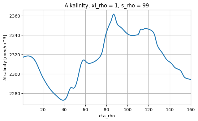
Or we specify a layer s and a xi slice.

[13]:

roms_output.plot("ALK", time=0, s=-1, xi=1)

[########################################] | 100% Completed | 101.81 ms

Plotting in lat/lon/depth coordinates#

Let’s now make a few plots in lat/lon/depth coordinates.

First we plot alkalinity at a 1000m depth.

[14]:

roms_output.plot("ALK", time=0, depth=1000)

[########################################] | 100% Completed | 101.91 ms

Here is a section of alkalinity along a fixed latitude of 20°N.

[15]:

roms_output.plot("ALK", time=0, lat=20)

[########################################] | 100% Completed | 101.88 ms

And here we plot along a fixed longitude of 120°W.

[16]:

roms_output.plot("ALK", time=0, lon=-120)

[########################################] | 100% Completed | 102.32 ms

We can also plot a vertical profile at a specified lat/lon location.

[17]:

roms_output.plot("ALK", time=0, lat=20, lon=-120)

[########################################] | 100% Completed | 102.18 ms

Or we plot at a fixed latitude and a fixed depth.

[18]:

roms_output.plot("ALK", time=0, lat=20, depth=1000)

[########################################] | 100% Completed | 101.75 ms

Plotting in native and lat/lon/depth coordinates combined#

Now we will use a combination of native dimensions and lat/lon/depth coordinates. However, note that

the horizontal native dimensions eta and xi cannot be combined with the horizontal coordinates lat and lon
the vertical native dimension s cannot be combined with the vertical coordinate depth.

In the next two plots we combine a horizontal lat/lon coordinate with the native vertical dimension s.

[19]:

roms_output.plot("ALK", time=0, lon=-120, s=-1)

[########################################] | 100% Completed | 102.14 ms

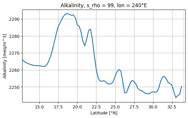
[20]:

roms_output.plot("ALK", time=0, lat=30, s=-1)

[########################################] | 100% Completed | 101.74 ms

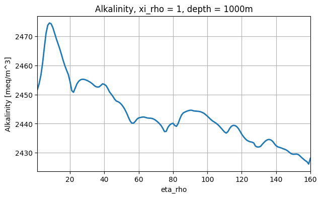
In the next two plots we combine a horizontal native dimension with a depth coordinate.

[21]:

roms_output.plot("ALK", time=0, eta=1, depth=1000)

[########################################] | 100% Completed | 101.82 ms

[22]:

roms_output.plot("ALK", time=0, xi=1, depth=1000)

[########################################] | 100% Completed | 101.83 ms

Handling the Horizontal Boundary#

The ROMSOutput.plot() method includes a parameter include_boundary, which controls whether the outermost grid cells along the eta- and xi-boundaries are included in the plot. In diagnostic ROMS output fields, these boundary cells are often set to zero, so excluding them can improve visualization.

By default, include_boundary = False, but we can set include_boundary = True to include the boundary cells in the plot.

Let’s plot the PH field, which is a diagnostic variable. The effect of these zeros along the horizontal boundary becomes evident in the next two plots.

[23]:

roms_output.plot("MARBL_PH_3D", time=0, s=-1, eta=1, include_boundary=True)

[########################################] | 100% Completed | 102.05 ms

The plot above confirms that the value at xi = 0 is zero.

Next, let’s plot the western boundary of the PH field by slicing along eta = 0. This boundary consists entirely of zeros.

[24]:

roms_output.plot("MARBL_PH_3D", time=0, s=-1, eta=0, include_boundary=True)

[########################################] | 100% Completed | 101.76 ms

Including the horizontal boundary for prognostic fields can lead to plots that are hard to read, as confirmed in the following.

[25]:

roms_output.plot("MARBL_PH_3D", time=0, s=-1, include_boundary=True)

[########################################] | 100% Completed | 101.58 ms

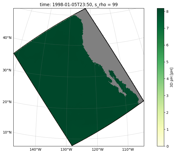
In the plot above, the colorbar extends down to zero due to a narrow band of zeros, one grid cell wide, along the boundary (although it is barely visible). This skewed colorbar makes it difficult to discern any features in the interior of the field.

When excluding the horizontal boundary, this problem is resolved, and the plot becomes much clearer.

[26]:

roms_output.plot("MARBL_PH_3D", time=0, s=-1, include_boundary=False)

[########################################] | 100% Completed | 101.82 ms

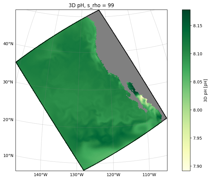
Note that you cannot exclude the horizontal boundary and request to plot the horizontal boundary at the same time. Doing so will result in an error.

[27]:

roms_output.plot("MARBL_PH_3D", time=0, s=-1, eta=0, include_boundary=False)

[########################################] | 100% Completed | 101.82 ms

---------------------------------------------------------------------------
ValueError                                Traceback (most recent call last)
Cell In[27], line 1
----> 1 roms_output.plot("MARBL_PH_3D", time=0, s=-1, eta=0, include_boundary=False)

File /anvil/projects/x-ees250129/x-smaticka/roms-tools/roms_tools/analysis/roms_output.py:210, in ROMSOutput.plot(self, var_name, time, s, eta, xi, depth, lat, lon, include_boundary, depth_contours, ax, save_path)
    207 else:
    208     cmap_name = "YlGn"
--> 210 plot(
    211     field=field,
    212     grid_ds=self.grid.ds,
    213     zeta=zeta,
    214     s=s,
    215     eta=eta,
    216     xi=xi,
    217     depth=depth,
    218     lat=lat,
    219     lon=lon,
    220     include_boundary=include_boundary,
    221     depth_contours=depth_contours,
    222     layer_contours=False,
    223     ax=ax,
    224     save_path=save_path,
    225     cmap_name=cmap_name,
    226 )

File /anvil/projects/x-ees250129/x-smaticka/roms-tools/roms_tools/plot.py:1311, in plot(field, grid_ds, zeta, s, eta, xi, depth, lat, lon, include_boundary, depth_contours, layer_contours, max_nr_layer_contours, yincrease, use_coarse_grid, with_dim_names, apply_mask, ax, save_path, cmap_name, add_colorbar)
   1191 def plot(
   1192     field: xr.DataArray,
   1193     grid_ds: xr.DataArray,
   (...)   1212     add_colorbar: bool = True,
   1213 ) -> None:
   1214     """Generate a plot of a 2D or 3D ROMS field for a horizontal or vertical slice.
   1215
   1216     This function supports plotting:
   (...)   1309         - If boundary indices are used when `include_boundary=False`.
   1310     """
-> 1311     prepared = prepare_field_for_plot(
   1312         field=field,
   1313         grid_ds=grid_ds,
   1314         zeta=zeta,
   1315         s=s,
   1316         eta=eta,
   1317         xi=xi,
   1318         depth=depth,
   1319         lat=lat,
   1320         lon=lon,
   1321         include_boundary=include_boundary,
   1322         depth_contours=depth_contours,
   1323         layer_contours=layer_contours,
   1324         max_nr_layer_contours=max_nr_layer_contours,
   1325         use_coarse_grid=use_coarse_grid,
   1326         with_dim_names=with_dim_names,
   1327         apply_mask=apply_mask,
   1328         cmap_name=cmap_name,
   1329     )
   1331     if prepared.plot_kind == "horizontal":
   1332         plot_2d_horizontal_field(
   1333             field=prepared.field,
   1334             depth_contours=prepared.depth_contours,
   (...)   1338             add_colorbar=add_colorbar,
   1339         )

File /anvil/projects/x-ees250129/x-smaticka/roms-tools/roms_tools/plot.py:856, in prepare_field_for_plot(field, grid_ds, zeta, s, eta, xi, depth, lat, lon, include_boundary, depth_contours, layer_contours, max_nr_layer_contours, use_coarse_grid, with_dim_names, apply_mask, cmap_name, lateral_regrid)
    835 def prepare_field_for_plot(
    836     field: xr.DataArray,
    837     grid_ds: xr.DataArray,
   (...)    853     lateral_regrid: Any = None,
    854 ) -> PreparedPlotField:
    855     """Prepare a single-time ROMS field for plotting (shared by ``plot`` and movies)."""
--> 856     _validate_plot_inputs(field, s, eta, xi, depth, lat, lon, include_boundary)
    858     if "straddle" not in grid_ds.attrs:
    859         raise AttributeError("Grid dataset must have a 'straddle' attribute.")

File /anvil/projects/x-ees250129/x-smaticka/roms-tools/roms_tools/plot.py:786, in _validate_plot_inputs(field, s, eta, xi, depth, lat, lon, include_boundary)
    784     if not include_boundary:
    785         if eta == 0 or eta == len(field[dim]) - 1:
--> 786             raise ValueError(
    787                 f"Invalid eta index: {eta} lies on the boundary, which is excluded when `include_boundary = False`. "
    788                 "Either set `include_boundary = True`, or adjust eta to avoid boundary values."
    789             )
    791 if xi is not None:
    792     dim = "xi_rho" if "xi_rho" in field.dims else "xi_u"

ValueError: Invalid eta index: 0 lies on the boundary, which is excluded when `include_boundary = False`. Either set `include_boundary = True`, or adjust eta to avoid boundary values.

Saving a Plot#

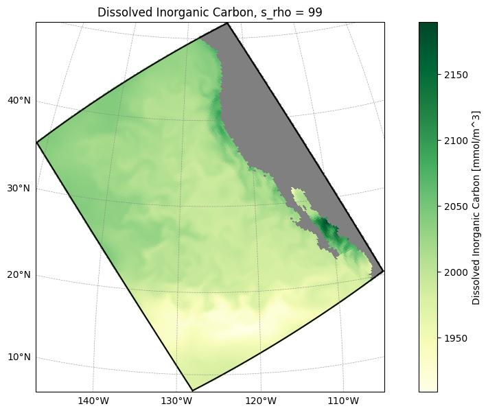
If you want to save a figure, you can specify the path using the save_path parameter when calling the .plot method.

[31]:

roms_output.plot("DIC", time=1, s=-1, save_path="figures/surface_DIC.png")

[########################################] | 100% Completed | 102.58 ms

Creating a Movie#

If you have many time steps loaded into ROMSOutput and ffmpeg is installed, you can use create_movie() to render an MP4 animation. It accepts the same spatial-selection and display parameters as .plot() — s, depth, eta, xi, lat, lon, include_boundary, depth_contours, use_coarse_grid, with_dim_names, and add_colorbar — but loops over time rather than plotting a single frame. You can restrict which time steps are animated with the time_range parameter (a slice or list of indices), control playback speed with fps, choose the output path with output_file, and add or reposition a timestamp overlay with timestamp_xy.

Note that only top-down horizontal map views are supported; vertical sections are not available in movies.

[28]:

# Create a movie of surface temperature over the first 24 time steps
roms_output.create_movie(
    var_name="temp",                 # RomsOutput data variable name (2D or 3D supported)
    time_range=slice(0, 24),         # animate time indices 0–23
    s=-1,                            # top layer (surface) (not required for 2D data variables)
    fps=8,                           # frames-per-second
    output_file="surface_temp.mp4",  # output filename
    timestamp_xy=(0.05, 0.95),       # (optional) axes-relative (x, y) position of the date/time label
)

[########################################] | 100% Completed | 102.37 ms

2026-06-16 20:14:40 - INFO - Animation.save using <class 'matplotlib.animation.FFMpegWriter'>
2026-06-16 20:14:40 - INFO - MovieWriter._run: running command: ffmpeg -f rawvideo -vcodec rawvideo -s 1300x700 -pix_fmt rgba -framerate 8 -loglevel error -i pipe: -vcodec libx264 -metadata artist=roms-tools -pix_fmt yuv420p -preset fast -y surface_temp.mp4

[########################################] | 100% Completed | 101.39 ms
[########################################] | 100% Completed | 101.78 ms
[########################################] | 100% Completed | 202.24 ms
[########################################] | 100% Completed | 202.87 ms
[########################################] | 100% Completed | 202.49 ms
Movie saved to surface_temp.mp4

[29]:

from IPython.display import Video

# Play a local MP4 file
Video("surface_temp.mp4", embed=True, width=640, height=360)

[29]:

[ ]: