Creating surface forcing

Creating surface forcing#

[2]:

from roms_tools import Grid, SurfaceForcing

/home/x-smaticka/.conda/envs/romstools-test/lib/python3.13/site-packages/tqdm/auto.py:21: TqdmWarning: IProgress not found. Please update jupyter and ipywidgets. See https://ipywidgets.readthedocs.io/en/stable/user_install.html
  from .autonotebook import tqdm as notebook_tqdm

As always, the first step is to create our grid. Let’s start with a coarse-resolution grid with a horizontal resolution of 2000km/100 = 20km.

[3]:

grid = Grid(
    nx=100,
    ny=100,
    size_x=2000,
    size_y=2000,
    center_lon=-18,
    center_lat=33,
    rot=-20,
    topography_source={
        "name": "SRTM15",
        "path": "/anvil/projects/x-ees250129/Datasets/SRTM15/SRTM15_V2.6.nc",
    },
)

Next, we specify the temporal range that we want to make the surface forcing for.

[4]:

from datetime import datetime

[5]:

start_time = datetime(2012, 1, 15)
end_time = datetime(2012, 2, 5)

ROMS-Tools can create three types of surface forcing:

physical surface forcing like 10m wind, shortwave radiation, and air temperature at 2m
biogeochemical (BGC) surface forcing like atmospheric dust or pCO2
restoring surface forcing like sea surface salinity

Unlike initial conditions data, ROMS can read multiple surface forcing files, so we create these three types separately in the following sections.

Physical surface forcing#

In this section, we use ERA5 data to construct the physical surface forcing. There are two ways to access the data:

Stream directly from the cloud (no download required)
Use locally pre-downloaded files by specifying the path

Streaming is convenient: there’s no need to download data in advance.

Local files, on the other hand, can reduce initialization time if you already have the data available.

Let’s explore both options with these keyword arguments:

[5]:

surface_forcing_kwargs = {
    "grid": grid,
    "start_time": start_time,
    "end_time": end_time,
    "type": "physics",
    "model_reference_date": datetime(2000, 1, 1), # this is the default
}

Streaming Cloud-based ERA5 Data#

Let’s begin by exploring the streaming approach. This method uses ARCO (Analysis-Ready, Cloud Optimized) ERA5 data from the public Google Cloud Storage bucket:

gs://gcp-public-data-arco-era5/ar/full_37-1h-0p25deg-chunk-1.zarr-v3

To activate the streaming approach in ROMS-Tools, simply omit the path in the source or explicitly provide the cloud storage URL:

source = {"name": "ERA5"}
source = {"name": "ERA5", "path": "gs://gcp-public-data-arco-era5/ar/full_37-1h-0p25deg-chunk-1.zarr-v3"}

Note

Streaming requires use_dask = True since the underlying data format is Zarr, which supports lazy loading and chunked access via Dask. Here you can learn more about using Dask with ROMS-Tools.

[6]:

%%time

surface_forcing = SurfaceForcing(
    **surface_forcing_kwargs,
    source={"name": "ERA5"},
    use_dask=True,
)

2026-05-21 14:28:24 - INFO - No path specified for ERA5 source; defaulting to ARCO ERA5 dataset on Google Cloud.
2026-05-21 14:29:36 - INFO - Data will be interpolated onto the fine grid. Remember to set `interp_frc = 0` in your `bulk_frc.opt` ROMS option file.

CPU times: user 1min 34s, sys: 16.3 s, total: 1min 50s
Wall time: 2min 12s

Instantiating the surface forcing took over 2 minutes, even though no computations have been performed yet due to Dask’s lazy evaluation. This delay results from streaming data from the cloud.

The surface forcing variables are held in an xarray.Dataset that is accessible via the .ds property. Indeed, all variables are Dask arrays representing lazy-loaded data.

[7]:

surface_forcing.ds

[7]:

<xarray.Dataset> Size: 148MB
Dimensions:   (time: 508, eta_rho: 102, xi_rho: 102)
Coordinates:
    abs_time  (time) datetime64[ns] 4kB 2012-01-14T23:00:00 ... 2012-02-05T02...
  * time      (time) float64 4kB 4.397e+03 4.397e+03 ... 4.418e+03 4.418e+03
    rad_time  (time) float64 4kB 4.397e+03 4.397e+03 ... 4.418e+03 4.418e+03
Dimensions without coordinates: eta_rho, xi_rho
Data variables:
    uwnd      (time, eta_rho, xi_rho) float32 21MB dask.array<chunksize=(1, 102, 102), meta=np.ndarray>
    vwnd      (time, eta_rho, xi_rho) float32 21MB dask.array<chunksize=(1, 102, 102), meta=np.ndarray>
    swrad     (time, eta_rho, xi_rho) float32 21MB dask.array<chunksize=(1, 102, 102), meta=np.ndarray>
    lwrad     (time, eta_rho, xi_rho) float32 21MB dask.array<chunksize=(1, 102, 102), meta=np.ndarray>
    Tair      (time, eta_rho, xi_rho) float32 21MB dask.array<chunksize=(1, 102, 102), meta=np.ndarray>
    rain      (time, eta_rho, xi_rho) float32 21MB dask.array<chunksize=(1, 102, 102), meta=np.ndarray>
    qair      (time, eta_rho, xi_rho) float32 21MB dask.array<chunksize=(1, 102, 102), meta=np.ndarray>
Attributes:
    title:                 ROMS surface forcing file created by ROMS-Tools
    roms_tools_version:    3.6.1.dev31+g34326e51e
    start_time:            2012-01-15 00:00:00
    end_time:              2012-02-05 00:00:00
    source:                ERA5
    correct_radiation:     True
    wind_dropoff:          False
    use_coarse_grid:       False
    model_reference_date:  2000-01-01 00:00:00
    type:                  physics

ROMS-Tools has found 508 time stamps within our specified time range. This includes time steps before and after the provided range, to allow ROMS to interpolate surface forcing data onto the start and end time points. Let’s double-check that ROMS-Tools has selected the correct times.

[8]:

surface_forcing.ds.time

Note

The time variable shows relative time, i.e., days since the model reference date (here set to January 1, 2000 by default). The abs_time coordinate shows the absolute time. The ERA5 data provided to ROMS-Tools has hourly frequency; this temporal frequency is inherited by surface_forcing.

To visualize any of the surface forcing fields, we can use the .plot method.

[9]:

surface_forcing.plot("uwnd", time=0)

[########################################] | 100% Completed | 101.65 ms

[10]:

surface_forcing.plot("swrad", time=15)

[########################################] | 100% Completed | 527.98 ms

Notice that the time corresponding to radiation is shifted from the 15\(^{th}\) element of abs_time by 30 minutes. This is because radiation fluxes are represented halfway through the timestep since they are an average over the timestep.

Using Local Pre-Downloaded ERA5 Data#

Next, let’s make the same surface forcing but using pre-downloaded ERA5 data sitting at the following location.

[11]:

path = "/anvil/projects/x-ees250129/Datasets/ERA5/NA/2012/ERA5*.nc"

You can also download your own ERA5 data, which must span the desired ROMS domain and temporal range. For more details, please refer to this page.

[12]:

%%time

surface_forcing_from_local_data = SurfaceForcing(
    **surface_forcing_kwargs,
    source={"name": "ERA5", "path": path},
    use_dask=True,
)

2026-05-21 14:45:41 - INFO - Data will be interpolated onto the fine grid. Remember to set `interp_frc = 0` in your `bulk_frc.opt` ROMS option file.

CPU times: user 2min 19s, sys: 12.1 s, total: 2min 31s
Wall time: 1min 29s

Instantiating the surface forcing was a little faster this time (~1.5 minutes) because it did not require streaming data.

[13]:

surface_forcing_from_local_data.ds

[13]:

<xarray.Dataset> Size: 148MB
Dimensions:   (time: 508, eta_rho: 102, xi_rho: 102)
Coordinates:
    abs_time  (time) datetime64[ns] 4kB 2012-01-14T23:00:00 ... 2012-02-05T02...
  * time      (time) float64 4kB 4.397e+03 4.397e+03 ... 4.418e+03 4.418e+03
    rad_time  (time) float64 4kB 4.397e+03 4.397e+03 ... 4.418e+03 4.418e+03
Dimensions without coordinates: eta_rho, xi_rho
Data variables:
    uwnd      (time, eta_rho, xi_rho) float32 21MB dask.array<chunksize=(1, 102, 102), meta=np.ndarray>
    vwnd      (time, eta_rho, xi_rho) float32 21MB dask.array<chunksize=(1, 102, 102), meta=np.ndarray>
    swrad     (time, eta_rho, xi_rho) float32 21MB dask.array<chunksize=(1, 102, 102), meta=np.ndarray>
    lwrad     (time, eta_rho, xi_rho) float32 21MB dask.array<chunksize=(1, 102, 102), meta=np.ndarray>
    Tair      (time, eta_rho, xi_rho) float32 21MB dask.array<chunksize=(1, 102, 102), meta=np.ndarray>
    rain      (time, eta_rho, xi_rho) float32 21MB dask.array<chunksize=(1, 102, 102), meta=np.ndarray>
    qair      (time, eta_rho, xi_rho) float32 21MB dask.array<chunksize=(1, 102, 102), meta=np.ndarray>
Attributes:
    title:                 ROMS surface forcing file created by ROMS-Tools
    roms_tools_version:    3.6.1.dev31+g34326e51e
    start_time:            2012-01-15 00:00:00
    end_time:              2012-02-05 00:00:00
    source:                ERA5
    correct_radiation:     True
    wind_dropoff:          False
    use_coarse_grid:       False
    model_reference_date:  2000-01-01 00:00:00
    type:                  physics

Horizontal regridding and source fill#

By default, physics surface forcing is regridded onto the ROMS grid with masked bilinear interpolation (using xESMF when available) plus inverse-distance-weighted extrapolation near coasts, so land/coastal points are filled with ocean-representative values without a separate whole-domain fill. When xESMF is not installed, ROMS-Tools falls back to a nearest-neighbor source pre-fill followed by SciPy linear interpolation.

Three optional arguments (shared with BoundaryForcing) control this:

``regrid_method`` — "auto" (default: xESMF if installed, else SciPy), "xesmf", or "scipy".
``prefill`` — fill the source over land before regridding. None (default) uses the masked-bilinear + extrapolation path above. Other options: "2d_lateral_fill" (the legacy AMG Poisson fill), "nearest_neighbor", "inverse_dist", "nearest_s2d", "creep_fill" (the last three require xESMF). Pass method-specific options via prefill_kwargs.
``extrap_method`` / ``extrap_kwargs`` — the destination extrapolation used on the default no-prefill path (defaults to "inverse_dist").

To reproduce the pre-v4 behavior exactly, pass prefill="2d_lateral_fill", regrid_method="scipy".

If the ROMS grid extends beyond the coverage of the source data, the default (extrapolating) path raises a coverage error rather than silently extrapolating — provide source data that covers the domain plus a margin.

These options apply to all SurfaceForcing types (physics, bgc, restoring). For bgc/restoring, the regression test fixtures are pinned to regrid_method="scipy" for byte-reproducibility, but the default is the masked-xESMF path as above.

Shortwave and longwave radiation correction#

Global data products like ERA5 are known to have biases in radiation, largely due to uncertainties in cloud-radiative feedbacks. To address these biases, ROMS-Tools includes a correction mechanism. When the correct_radiation parameter is set to True (which is the default), multiplicative correction factors are applied to both the ERA5 shortwave and downwelling longwave radiation data. These correction factors are pre-computed based on the difference between ERA5 climatology and the COREv2 climatology.

As a result, the surface_forcing dataset we generated above includes shortwave and longwave radiation corrections, since the default setting for correct_radiation is True. In the following, we create surface forcing where no correction is applied. While this approach is possible, it is not recommended due to the known biases in the ERA5 radiation data.

[14]:

%%time

uncorrected_surface_forcing = SurfaceForcing(
    grid=grid,
    start_time=start_time,
    end_time=end_time,
    source={"name": "ERA5", "path": path},
    type="physics",
    correct_radiation=False,  # default is True
    use_dask=True,
)

2026-05-21 14:47:09 - INFO - Data will be interpolated onto the fine grid. Remember to set `interp_frc = 0` in your `bulk_frc.opt` ROMS option file.

CPU times: user 2min 10s, sys: 12.1 s, total: 2min 22s
Wall time: 1min 20s

[15]:

uncorrected_surface_forcing.ds

[15]:

<xarray.Dataset> Size: 148MB
Dimensions:   (time: 508, eta_rho: 102, xi_rho: 102)
Coordinates:
    abs_time  (time) datetime64[ns] 4kB 2012-01-14T23:00:00 ... 2012-02-05T02...
  * time      (time) float64 4kB 4.397e+03 4.397e+03 ... 4.418e+03 4.418e+03
    rad_time  (time) float64 4kB 4.397e+03 4.397e+03 ... 4.418e+03 4.418e+03
Dimensions without coordinates: eta_rho, xi_rho
Data variables:
    uwnd      (time, eta_rho, xi_rho) float32 21MB dask.array<chunksize=(1, 102, 102), meta=np.ndarray>
    vwnd      (time, eta_rho, xi_rho) float32 21MB dask.array<chunksize=(1, 102, 102), meta=np.ndarray>
    swrad     (time, eta_rho, xi_rho) float32 21MB dask.array<chunksize=(1, 102, 102), meta=np.ndarray>
    lwrad     (time, eta_rho, xi_rho) float32 21MB dask.array<chunksize=(1, 102, 102), meta=np.ndarray>
    Tair      (time, eta_rho, xi_rho) float32 21MB dask.array<chunksize=(1, 102, 102), meta=np.ndarray>
    rain      (time, eta_rho, xi_rho) float32 21MB dask.array<chunksize=(1, 102, 102), meta=np.ndarray>
    qair      (time, eta_rho, xi_rho) float32 21MB dask.array<chunksize=(1, 102, 102), meta=np.ndarray>
Attributes:
    title:                 ROMS surface forcing file created by ROMS-Tools
    roms_tools_version:    3.6.1.dev31+g34326e51e
    start_time:            2012-01-15 00:00:00
    end_time:              2012-02-05 00:00:00
    source:                ERA5
    correct_radiation:     False
    wind_dropoff:          False
    use_coarse_grid:       False
    model_reference_date:  2000-01-01 00:00:00
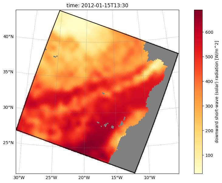
    type:                  physics

Here is a plot of the downward short-wave radiation, as before, but now in its uncorrected version. The downwelling longwave radiation is similarly uncorrected when correct_radiation=False.

[16]:

uncorrected_surface_forcing.plot("swrad", time=15)

[########################################] | 100% Completed | 203.27 ms

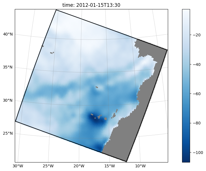
Let’s plot the differences in corrected and uncorrected short-wave radiation. Analogous differences apply to the downwelling longwave radiation.

[17]:

from roms_tools.plot import plot

[18]:

plot(
    (surface_forcing.ds["swrad"] - uncorrected_surface_forcing.ds["swrad"]).isel(
        time=15
    ),
    grid_ds=grid.ds,
    cmap_name="Blues_r",
)

Wind Correction Near the Coast#

ERA5’s 1/4° resolution is too coarse to capture realistic coastal winds, particularly the wind drop-off near the coast. This drop-off is caused by coastal orography and differences between marine and terrestrial surface layers. It plays a crucial dynamical role in coastal upwelling systems, where the wind stress curl in the drop-off zone significantly influences Ekman pumping and biogeochemical reaction rates.

To address this limitation, ROMS-Tools can apply an exponential reduction in wind magnitude near the coastline. This correction uses an e-folding scale of 12.5 km, smoothly transitioning from full offshore wind strength to a 40% reduction at the shore. The behavior is controlled by the wind_dropoff parameter, which is set to False by default.

[19]:

surface_forcing_with_wind_drop_off = SurfaceForcing(
    grid=grid,
    start_time=start_time,
    end_time=end_time,
    source={"name": "ERA5", "path": path},
    type="physics",
    wind_dropoff=True,
    use_dask=True,
)

2026-05-21 14:48:35 - INFO - Data will be interpolated onto the fine grid. Remember to set `interp_frc = 0` in your `bulk_frc.opt` ROMS option file.

[20]:

surface_forcing_with_wind_drop_off.ds

[20]:

<xarray.Dataset> Size: 148MB
Dimensions:   (time: 508, eta_rho: 102, xi_rho: 102)
Coordinates:
    abs_time  (time) datetime64[ns] 4kB 2012-01-14T23:00:00 ... 2012-02-05T02...
  * time      (time) float64 4kB 4.397e+03 4.397e+03 ... 4.418e+03 4.418e+03
    rad_time  (time) float64 4kB 4.397e+03 4.397e+03 ... 4.418e+03 4.418e+03
Dimensions without coordinates: eta_rho, xi_rho
Data variables:
    uwnd      (time, eta_rho, xi_rho) float32 21MB dask.array<chunksize=(1, 102, 102), meta=np.ndarray>
    vwnd      (time, eta_rho, xi_rho) float32 21MB dask.array<chunksize=(1, 102, 102), meta=np.ndarray>
    swrad     (time, eta_rho, xi_rho) float32 21MB dask.array<chunksize=(1, 102, 102), meta=np.ndarray>
    lwrad     (time, eta_rho, xi_rho) float32 21MB dask.array<chunksize=(1, 102, 102), meta=np.ndarray>
    Tair      (time, eta_rho, xi_rho) float32 21MB dask.array<chunksize=(1, 102, 102), meta=np.ndarray>
    rain      (time, eta_rho, xi_rho) float32 21MB dask.array<chunksize=(1, 102, 102), meta=np.ndarray>
    qair      (time, eta_rho, xi_rho) float32 21MB dask.array<chunksize=(1, 102, 102), meta=np.ndarray>
Attributes:
    title:                 ROMS surface forcing file created by ROMS-Tools
    roms_tools_version:    3.6.1.dev31+g34326e51e
    start_time:            2012-01-15 00:00:00
    end_time:              2012-02-05 00:00:00
    source:                ERA5
    correct_radiation:     True
    wind_dropoff:          True
    use_coarse_grid:       False
    model_reference_date:  2000-01-01 00:00:00
    type:                  physics

Here is a plot of the zonal wind, as before, but now with reduced amplitude near the coasts.

[21]:

surface_forcing_with_wind_drop_off.plot("uwnd", time=0)

[########################################] | 100% Completed | 103.95 ms

Here is the difference between the uncorrected and corrected wind.

[22]:

plot(
    (surface_forcing.ds["uwnd"] - surface_forcing_with_wind_drop_off.ds["uwnd"]).isel(
        time=0
    ),
    grid_ds=grid.ds,
    cmap_name="RdBu_r",
)

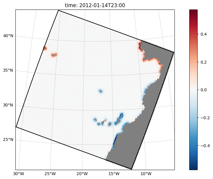
The plot above highlights differences concentrated in near-coastal areas. Comparing the sign of the difference plot with the original wind field shows that positive wind values have been reduced and negative values enhanced, indicating a consistent reduction in wind amplitude near the coast.

Fine vs. coarse grid#

ROMS-Tools provides the option to interpolate surface forcing fields onto a “coarse grid,” which has a resolution that is a factor of 2 coarser than the original “fine grid.” Interpolating onto the coarse grid is useful when the ROMS grid resolution is at least twice as fine as that of the raw data product (e.g., ERA5). In such cases, interpolating onto the fine grid would not provide additional information compared to the coarse grid, making the coarse grid a more efficient choice and saving computational resources.

To control the choice between fine and coarse grids, ROMS-Tools provides the coarse_grid_mode argument, which accepts the following options:

“auto” (default): Automatically selects the appropriate grid based on the comparison of the source and target spatial resolutions.
“always”: Always interpolate onto the coarse grid.
“never”: Always interpolate onto the fine grid, bypassing the coarse grid.

ROMS-Tools generates an informational message to indicate whether the fine or coarse grid is being used.

The surface forcings we have generated so far have used coarse_grid_mode = "auto", and the info messages indicated that the fine grid was selected. This decision was made because the ROMS grid resolution of approximately 20 km is similar to the ERA5 resolution of 1/4° (which at 33°N is about 23 km) - not fine enough to warrant using the coarse grid.

Now, let’s try using a grid with a higher resolution of 2000km/200 = 10km.

[23]:

grid_10km = Grid(
    nx=200,
    ny=200,
    size_x=2000,
    size_y=2000,
    center_lon=-18,
    center_lat=33,
    rot=-20,
    topography_source={
        "name": "SRTM15",
        "path": "/anvil/projects/x-ees250129/Datasets/SRTM15/SRTM15_V2.6.nc",
    },
)

[24]:

grid_10km.ds

[25]:

%%time

surface_forcing_for_grid_10km = SurfaceForcing(
    grid=grid_10km,
    start_time=start_time,
    end_time=end_time,
    source={"name": "ERA5", "path": path},
    type="physics",
    coarse_grid_mode="auto",  # default is "auto"
    use_dask=True,
)

2026-05-21 14:50:16 - INFO - Data will be interpolated onto the grid coarsened by factor 2. Remember to set `interp_frc = 1` in your `bulk_frc.opt` ROMS option file.

CPU times: user 2min 2s, sys: 13.5 s, total: 2min 16s
Wall time: 1min 30s

The info message confirms that ROMS-Tools has interpolated onto the “coarse grid,” as the coarsened 10 km grid has a resolution of 20 km, which is still finer than the ERA5 resolution.

[26]:

surface_forcing_for_grid_10km.ds

[26]:

<xarray.Dataset> Size: 148MB
Dimensions:   (time: 508, eta_rho: 102, xi_rho: 102)
Coordinates:
    abs_time  (time) datetime64[ns] 4kB 2012-01-14T23:00:00 ... 2012-02-05T02...
  * time      (time) float64 4kB 4.397e+03 4.397e+03 ... 4.418e+03 4.418e+03
    rad_time  (time) float64 4kB 4.397e+03 4.397e+03 ... 4.418e+03 4.418e+03
Dimensions without coordinates: eta_rho, xi_rho
Data variables:
    uwnd      (time, eta_rho, xi_rho) float32 21MB dask.array<chunksize=(1, 102, 102), meta=np.ndarray>
    vwnd      (time, eta_rho, xi_rho) float32 21MB dask.array<chunksize=(1, 102, 102), meta=np.ndarray>
    swrad     (time, eta_rho, xi_rho) float32 21MB dask.array<chunksize=(1, 102, 102), meta=np.ndarray>
    lwrad     (time, eta_rho, xi_rho) float32 21MB dask.array<chunksize=(1, 102, 102), meta=np.ndarray>
    Tair      (time, eta_rho, xi_rho) float32 21MB dask.array<chunksize=(1, 102, 102), meta=np.ndarray>
    rain      (time, eta_rho, xi_rho) float32 21MB dask.array<chunksize=(1, 102, 102), meta=np.ndarray>
    qair      (time, eta_rho, xi_rho) float32 21MB dask.array<chunksize=(1, 102, 102), meta=np.ndarray>
Attributes:
    title:                 ROMS surface forcing file created by ROMS-Tools
    roms_tools_version:    3.6.1.dev31+g34326e51e
    start_time:            2012-01-15 00:00:00
    end_time:              2012-02-05 00:00:00
    source:                ERA5
    correct_radiation:     True
    wind_dropoff:          False
    use_coarse_grid:       True
    model_reference_date:  2000-01-01 00:00:00
    type:                  physics

As expected, the lengths of the spatial dimensions eta_rho and xi_rho in the surface forcing dataset are now 102—half of their original lengths of 202 in the fine grid, and equal to the lengths of eta_coarse and xi_coarse in the grid dataset.

Note

The dimension names in surface_forcing_for_grid_10km.ds are somewhat confusingly called eta_rho, xi_rho (rather than eta_coarse, xi_coarse). This is due to a particularity of ROMS - it expects the dimension names eta_rho, xi_rho even if the coarse grid is used.

We could also force interpolation onto the fine grid, though this would unnecessarily increase computational cost without adding any additional information.

[27]:

%%time

fine_surface_forcing_for_grid_10km = SurfaceForcing(
    grid=grid_10km,
    start_time=start_time,
    end_time=end_time,
    source={"name": "ERA5", "path": path},
    type="physics",
    coarse_grid_mode="never",
    use_dask=True,
)

2026-05-21 14:51:47 - INFO - Data will be interpolated onto the fine grid. Remember to set `interp_frc = 0` in your `bulk_frc.opt` ROMS option file.

CPU times: user 2min 7s, sys: 13.6 s, total: 2min 20s
Wall time: 1min 32s

[28]:

fine_surface_forcing_for_grid_10km.ds

[28]:

<xarray.Dataset> Size: 580MB
Dimensions:   (time: 508, eta_rho: 202, xi_rho: 202)
Coordinates:
    abs_time  (time) datetime64[ns] 4kB 2012-01-14T23:00:00 ... 2012-02-05T02...
  * time      (time) float64 4kB 4.397e+03 4.397e+03 ... 4.418e+03 4.418e+03
    rad_time  (time) float64 4kB 4.397e+03 4.397e+03 ... 4.418e+03 4.418e+03
Dimensions without coordinates: eta_rho, xi_rho
Data variables:
    uwnd      (time, eta_rho, xi_rho) float32 83MB dask.array<chunksize=(1, 202, 202), meta=np.ndarray>
    vwnd      (time, eta_rho, xi_rho) float32 83MB dask.array<chunksize=(1, 202, 202), meta=np.ndarray>
    swrad     (time, eta_rho, xi_rho) float32 83MB dask.array<chunksize=(1, 202, 202), meta=np.ndarray>
    lwrad     (time, eta_rho, xi_rho) float32 83MB dask.array<chunksize=(1, 202, 202), meta=np.ndarray>
    Tair      (time, eta_rho, xi_rho) float32 83MB dask.array<chunksize=(1, 202, 202), meta=np.ndarray>
    rain      (time, eta_rho, xi_rho) float32 83MB dask.array<chunksize=(1, 202, 202), meta=np.ndarray>
    qair      (time, eta_rho, xi_rho) float32 83MB dask.array<chunksize=(1, 202, 202), meta=np.ndarray>
Attributes:
    title:                 ROMS surface forcing file created by ROMS-Tools
    roms_tools_version:    3.6.1.dev31+g34326e51e
    start_time:            2012-01-15 00:00:00
    end_time:              2012-02-05 00:00:00
    source:                ERA5
    correct_radiation:     True
    wind_dropoff:          False
    use_coarse_grid:       False
    model_reference_date:  2000-01-01 00:00:00
    type:                  physics

The spatial dimensions eta_rho and xi_rho in the surface forcing dataset remain 202, matching their original lengths in the grid_10km.

Biogeochemical (BGC) surface forcing#

We now generate BGC surface forcing by interpolating biogeochemical variables from a dataset with 1° horizontal resolution. For our approach we use:

A Unified BGC Climatology, which integrates observationally and model based sources:

Atmospheric pCO₂ from [Landschützer et al., 2016]
Iron, dust, NOx and NHy decompositions from CESM model simulations

The BGC dataset is available at the following location:

[1]:

unified_bgc_path = "/anvil/projects/x-ees250129/Datasets/UNIFIED/BGCdataset.nc"

[32]:

%%time

unified_bgc_surface_forcing = SurfaceForcing(
    grid=grid,
    start_time=start_time,
    end_time=end_time,
    source={"name": "UNIFIED", "path": unified_bgc_path, "climatology": True},
    type="bgc",
    use_dask=True,
)

2026-05-21 14:55:15 - INFO - Data will be interpolated onto the grid coarsened by factor 2. Remember to set `interp_frc = 1` in your `bgc.opt` ROMS option file.

CPU times: user 103 ms, sys: 6.86 ms, total: 110 ms
Wall time: 145 ms

[33]:

unified_bgc_surface_forcing.ds

[33]:

<xarray.Dataset> Size: 520kB
Dimensions:    (time: 12, eta_rho: 52, xi_rho: 52)
Coordinates:
    month      (time) int64 96B 1 2 3 4 5 6 7 8 9 10 11 12
    abs_time   (time) datetime64[ns] 96B 2000-01-16T12:00:00 ... 2000-12-15T1...
    iron_time  (time) float64 96B 15.5 45.0 74.5 105.0 ... 288.5 319.0 349.5
    dust_time  (time) float64 96B 15.5 45.0 74.5 105.0 ... 288.5 319.0 349.5
    nox_time   (time) float64 96B 15.5 45.0 74.5 105.0 ... 288.5 319.0 349.5
    nhy_time   (time) float64 96B 15.5 45.0 74.5 105.0 ... 288.5 319.0 349.5
Dimensions without coordinates: time, eta_rho, xi_rho
Data variables:
    dust       (time, eta_rho, xi_rho) float32 130kB dask.array<chunksize=(1, 52, 52), meta=np.ndarray>
    iron       (time, eta_rho, xi_rho) float32 130kB dask.array<chunksize=(1, 52, 52), meta=np.ndarray>
    nox        (time, eta_rho, xi_rho) float32 130kB dask.array<chunksize=(1, 52, 52), meta=np.ndarray>
    nhy        (time, eta_rho, xi_rho) float32 130kB dask.array<chunksize=(1, 52, 52), meta=np.ndarray>
Attributes:
    title:                 ROMS surface forcing file created by ROMS-Tools
    roms_tools_version:    3.6.1.dev31+g34326e51e
    start_time:            2012-01-15 00:00:00
    end_time:              2012-02-05 00:00:00
    source:                UNIFIED
    correct_radiation:     True
    wind_dropoff:          False
    use_coarse_grid:       True
    model_reference_date:  2000-01-01 00:00:00
    type:                  bgc
    climatology:           True

Note

Unified BGC Climatology: Since this dataset is climatological (source["climatology"] = True), it always contains twelve time entries, unaffected by start_time and end_time. All *_time coordinates include a cycle_length attribute (in days), instructing ROMS to repeat the data every 365.25 days. This makes unified_bgc_boundary_forcing.ds suitable for any simulation period, provided the reference date is January 1 of any year.

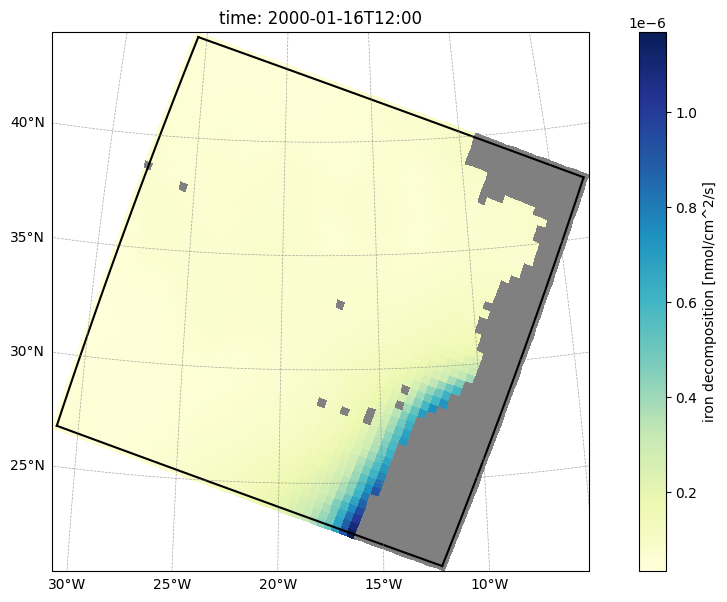
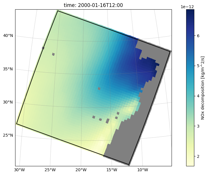
We can plot the BGC surface forcing as we saw above.

[35]:

unified_bgc_surface_forcing.plot("iron", time=0)

[########################################] | 100% Completed | 101.33 ms

[37]:

unified_bgc_surface_forcing.plot("nox", time=0)

[########################################] | 100% Completed | 101.82 ms

Time-varying CO2#

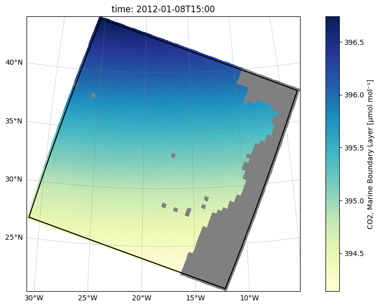
By default, ROMS assumes a constant value for the molar mixing ratio for CO2, xco2. If we would like a time-varying xco2 applied in the model, we can create a BGC surface forcing object containing xco2, similar to the BGC surface forcing generated above.

The xco2 data is interpolated from the GML’s (NOAA) Marine Boundary Layer dataset (1979-2025). There are two ways to access the data:

Stream directly from a URL (no download required); The data to be stream is small, so this is a convenient and fast method
Use locally pre-downloaded files by specifying the path

Note

By default ROMS will use a constant value for xco2. In order to best model the carbonate system during a CDR release, it is ideal to use a time-varying atmospheric CO₂ record.

Since climatological data represents a single value for each month and is repeated annually, it is appropriate for slowly-varying BGC forces, whose interannual variability is small relative to their biogeochemical effect. Because CDR release simulations depend on accurately resolving the air-sea pCO₂ gradient, ROMS-Tools supports time-varying xco2 derived from the NOAA Marine Boundary Layer (MBL) product, an observationally-grounded dataset, to best represent the true atmospheric boundary conditions.

Streaming MBL Data#

Similar to the ERA5 streaming approach, to activate the streaming, simply omit the path in the source or explicitly provide the URL: "https://gml.noaa.gov/ccgg/mbl/tmp/co2_GHGreference.1785677502_surface.txt"

This method uses the data available from NOAA’s GML Marine Boundary Layer Reference, which is available as a function of latitude. Therefore, the value for xco2 is assumed to be held constant for all longitudes.

source = {"name": "MBL_co2"}
source = {"name": "MBL_co2", "path": "https://gml.noaa.gov/ccgg/mbl/tmp/co2_GHGreference.1785677502_surface.txt"}

[38]:

%%time

mbl_bgc_surface_forcing = SurfaceForcing(
    grid=grid,
    start_time=start_time,
    end_time=end_time,
    source={"name": "MBL_co2"},
    type="bgc",
)

2026-05-21 15:09:17 - INFO - No path specified for MBL_co2 source; defaulting to the MBL dataset from GML, NOAA.
2026-05-21 15:09:17 - INFO - Data will be interpolated onto the grid coarsened by factor 2. Remember to set `interp_frc = 1` in your `bgc.opt` ROMS option file.
2026-05-21 15:09:17 - INFO - Time-varying CO2 values being used.Remember to define the following flags in your `cppdefs.opt` file: {'PCO2AIR_FORCING'}`.

CPU times: user 53.6 ms, sys: 15 ms, total: 68.5 ms
Wall time: 95.3 ms

Local MBL Data#

To use a pre-downloaded file, provide the path:

[39]:

MBL_path = "/anvil/projects/x-ees250129/Datasets/MBL/co2_GHGreference.1785677502_surface.txt"

[40]:

%%time

mbl_bgc_surface_forcing_local_data = SurfaceForcing(
    grid=grid,
    start_time=start_time,
    end_time=end_time,
    source={"name": "MBL_co2", "path": MBL_path},
    type="bgc",
)

2026-05-21 15:32:22 - INFO - Data will be interpolated onto the grid coarsened by factor 2. Remember to set `interp_frc = 1` in your `bgc.opt` ROMS option file.
2026-05-21 15:32:22 - INFO - Time-varying CO2 values being used.Remember to define the following flags in your `cppdefs.opt` file: {'PCO2AIR_FORCING'}`.

CPU times: user 59.1 ms, sys: 11.9 ms, total: 71 ms
Wall time: 99 ms

[41]:

mbl_bgc_surface_forcing.plot("xco2_air", time=0)

Restoring surface forces#

Finally, we generate a restoring surface forces file. Restoring is used to prevent the model from drifting over time by applying a small nudge or correction to specific variables. Variables that can be prescribed for restoration in ROMS are sea surface salinity (sss), DIC (sDIC), and ALK (sALK).

To turn on restoring forces in ROMS, the following flags need to be defined in the cppdefs.opt file, according to the variable to be restored:

Salinity: SFLX_CORR
DIC & ALK: CFLX_COR

For salinity, two data sources are available:

World Ocean Atlas data, which is a gridded set of observations taken from profile data.
- Instructions for downloading this data can be found in the Datasets section.
- In this example, we use the WOA 2018 1/4° horizontal resolution, found here (labels: s01-s12).
The Unified BGC Climatology discussed above includes sea surface salinity taken from the 2018 World Ocean Atlas. This data has 1° horizontal resolution.

For DIC and ALK, we use:

The OceanSODA dataset from NOAA’s NCEI. It is a global gridded marine carbonate system dataset calculated from machine learning estimates.
- Instructions for downloading this data is found in the Datasets section.

Note

Because sea surface salinity (sss) is pulled from climatological data, and the sea surface DIC (sDIC) and Alkalinity (sALK) are pulled from monthly data, the SurfaceForcing class needs to be called once for sss and once for sDIC & sALK. This results in one file for sss and one file for sDIC & sALK.

Salinity Restoring#

[42]:

woa_restoring_path = "/anvil/projects/x-ees250129/Datasets/WOA/2018/woa18_decav_s*_04.nc"
unified_bgc_path = "/anvil/projects/x-ees250129/Datasets/UNIFIED/BGCdataset.nc"

[43]:

%%time

woa_restoring_surface_forcing = SurfaceForcing(
    grid=grid,
    start_time=start_time,
    end_time=end_time,
    source={"name": "WOA", "path": woa_restoring_path, "climatology": True},
    type="restoring",
    restoring_forces=['sss'],
    use_dask=True,
)

2026-06-22 20:58:39 - INFO - Data will be interpolated onto the fine grid. Restoring data being created for ['sss']. Remember to define the following flags in your `cppdefs.opt` file: {'SFLX_CORR'}`.

CPU times: user 3min 40s, sys: 348 ms, total: 3min 41s
Wall time: 10.5 s

[44]:

woa_restoring_surface_forcing.ds

[44]:

<xarray.Dataset> Size: 500kB
Dimensions:   (time: 12, eta_rho: 102, xi_rho: 102)
Coordinates:
    month     (time) int64 96B 1 2 3 4 5 6 7 8 9 10 11 12
    abs_time  (time) datetime64[ns] 96B 2000-01-16 2000-02-15 ... 2000-12-15
    sss_time  (time) float64 96B 15.0 45.0 74.0 105.0 ... 288.0 319.0 349.0
Dimensions without coordinates: time, eta_rho, xi_rho
Data variables:
    sss       (time, eta_rho, xi_rho) float32 499kB dask.array<chunksize=(1, 102, 102), meta=np.ndarray>
Attributes:
    title:                 ROMS surface forcing file created by ROMS-Tools
    roms_tools_version:    3.6.1.dev31+g34326e51e
    start_time:            2012-01-15 00:00:00
    end_time:              2012-02-05 00:00:00
    source:                WOA
    correct_radiation:     True
    wind_dropoff:          False
    use_coarse_grid:       False
    model_reference_date:  2000-01-01 00:00:00
    type:                  restoring
    climatology:           True

[45]:

%%time

unified_restoring_surface_forcing = SurfaceForcing(
    grid=grid,
    start_time=start_time,
    end_time=end_time,
    source={"name": "UNIFIED", "path": unified_bgc_path, "climatology": True},
    type="restoring",
    restoring_forces=['sss'],
    use_dask=True,
)

2026-05-21 15:30:59 - INFO - Data will be interpolated onto the grid coarsened by factor 2. Restoring data being created for ['sss']. Remember to define the following flags in your `cppdefs.opt` file: {'SFLX_CORR'}`.

CPU times: user 79.4 ms, sys: 4.96 ms, total: 84.3 ms
Wall time: 82.9 ms

[46]:

unified_restoring_surface_forcing.ds

[46]:

<xarray.Dataset> Size: 130kB
Dimensions:   (time: 12, eta_rho: 52, xi_rho: 52)
Coordinates:
    month     (time) int64 96B 1 2 3 4 5 6 7 8 9 10 11 12
    abs_time  (time) datetime64[ns] 96B 2000-01-16T12:00:00 ... 2000-12-15T12...
    sss_time  (time) float64 96B 15.5 45.0 74.5 105.0 ... 288.5 319.0 349.5
Dimensions without coordinates: time, eta_rho, xi_rho
Data variables:
    sss       (time, eta_rho, xi_rho) float32 130kB dask.array<chunksize=(1, 52, 52), meta=np.ndarray>
Attributes:
    title:                 ROMS surface forcing file created by ROMS-Tools
    roms_tools_version:    3.6.1.dev31+g34326e51e
    start_time:            2012-01-15 00:00:00
    end_time:              2012-02-05 00:00:00
    source:                UNIFIED
    correct_radiation:     True
    wind_dropoff:          False
    use_coarse_grid:       True
    model_reference_date:  2000-01-01 00:00:00
    type:                  restoring
    climatology:           True

Note

Since WOA data is climatological (source["climatology"] = True), similar to the Unified BGC data, the generated dataset always contains twelve time entries, unaffected by start_time and end_time. All *_time coordinates include a cycle_length attribute (in days), instructing ROMS to repeat the data every 365.25 days. This makes unified_restoring_surface_forcing.ds suitable for any simulation period, provided the reference date is January 1 of any year.

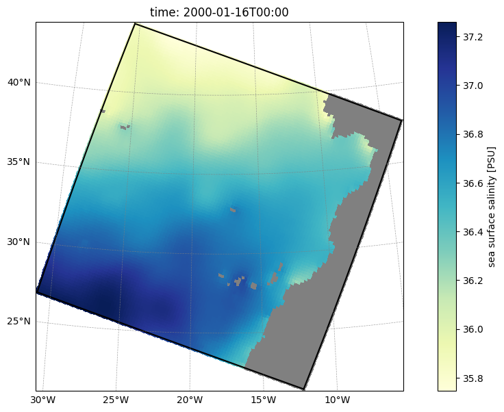
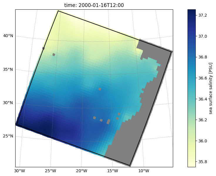
We can plot the restoring force for each data source.

[47]:

woa_restoring_surface_forcing.plot("sss", time=0)

[########################################] | 100% Completed | 309.50 ms

[48]:

unified_restoring_surface_forcing.plot("sss", time=0)

[########################################] | 100% Completed | 101.53 ms

Saving as NetCDF or YAML file#

Once we have decided which of the surface forcing versions we actually want to use, we can save the dataset as a NetCDF file.

We need to specify the desired target path.

[54]:

filepath = "/anvil/scratch/x-smaticka/forcing/my_bgc_surface_forcing.nc"

[55]:

%time unified_bgc_surface_forcing.save(filepath)

2026-05-21 15:31:17 - INFO - Writing the following NetCDF files:
/anvil/scratch/x-smaticka/forcing/my_bgc_surface_forcing_2012.nc

[########################################] | 100% Completed | 307.48 ms
CPU times: user 183 ms, sys: 145 ms, total: 328 ms
Wall time: 371 ms

[55]:

[PosixPath('/anvil/scratch/x-smaticka/forcing/my_bgc_surface_forcing_2012.nc')]

[56]:

filepath = "/anvil/scratch/x-smaticka/forcing/my_co2_surface_forcing.nc"

[57]:

%time mbl_bgc_surface_forcing.save(filepath)

2026-05-21 15:32:42 - INFO - Writing the following NetCDF files:
/anvil/scratch/x-smaticka/forcing/my_co2_surface_forcing_2012.nc

CPU times: user 7.2 ms, sys: 965 μs, total: 8.17 ms
Wall time: 9.69 ms

[57]:

[PosixPath('/anvil/scratch/x-smaticka/forcing/my_co2_surface_forcing_2012.nc')]

[58]:

filepath = "/anvil/scratch/x-smaticka/forcing/my_restoring_forces_SSS.nc"

[59]:

%time woa_restoring_surface_forcing.save(filepath)

2026-06-22 20:58:48 - INFO - Writing the following NetCDF files:
/anvil/scratch/x-smaticka/forcing/my_restoring_forces_SSS_clim.nc

[########################################] | 100% Completed | 621.13 ms
CPU times: user 11.9 s, sys: 109 ms, total: 12 s
Wall time: 724 ms

[59]:

[PosixPath('/anvil/scratch/x-smaticka/forcing/my_restoring_forces_SSS_clim.nc')]

[60]:

filepath = "/anvil/scratch/x-smaticka/forcing/my_restoring_forces_DIC_ALK.nc"

[61]:

%time soda_restoring_surface_forcing_local.save(filepath)

2026-05-21 15:31:19 - INFO - Writing the following NetCDF files:
/anvil/scratch/x-smaticka/forcing/my_restoring_forces_clim.nc

[########################################] | 100% Completed | 514.44 ms
CPU times: user 7.47 s, sys: 89.1 ms, total: 7.56 s
Wall time: 605 ms

[61]:

[PosixPath('/anvil/scratch/x-smaticka/forcing/my_restoring_forces_clim.nc')]

Alternatively, we can tell ROMS-Tools to group the surface forcing into multiple files ordered by months.

[62]:

filepath = "/anvil/scratch/x-smaticka/forcing/my_surface_forcing.nc"

[63]:

%time surface_forcing.save(filepath, group=True)

2026-05-21 15:31:22 - INFO - Writing the following NetCDF files:
/anvil/scratch/x-smaticka/forcing/my_surface_forcing_201201.nc
/anvil/scratch/x-smaticka/forcing/my_surface_forcing_201202.nc

[########################################] | 100% Completed | 36.74 s
[########################################] | 100% Completed | 9.23 sms
CPU times: user 27min 39s, sys: 6.75 s, total: 27min 45s
Wall time: 48.7 s

[63]:

[PosixPath('/anvil/scratch/x-smaticka/forcing/my_surface_forcing_201201.nc'),
 PosixPath('/anvil/scratch/x-smaticka/forcing/my_surface_forcing_201202.nc')]

From the file paths printed to the screen, you will notice that the year and month information has been appended to the specified path.

Note

The way data is grouped depends on its temporal frequency. For datasets with a daily or higher frequency, the data is grouped by month. For datasets with lower temporal frequency (e.g., monthly data), the grouping is done by year.

We can also export the parameters of our SurfaceForcing object to a YAML file.

[64]:

yaml_filepath = "/anvil/scratch/x-smaticka/forcing/my_surface_forcing.yaml"

[65]:

surface_forcing.to_yaml(yaml_filepath)

This is the YAML file that was created.

[66]:

# Open and read the YAML file
with open(yaml_filepath, "r") as file:
    file_contents = file.read()

# Print the contents
print(file_contents)

---
roms_tools_version: 3.6.1.dev31+g34326e51e
---
Grid:
  nx: 100
  ny: 100
  size_x: 2000
  size_y: 2000
  center_lon: -18
  center_lat: 33
  rot: -20
  N: 100
  theta_s: 5.0
  theta_b: 2.0
  hc: 300.0
  topography_source:
    name: SRTM15
    path: /anvil/projects/x-ees250129/Datasets/SRTM15/SRTM15_V2.6.nc
  mask_shapefile: null
  close_narrow_channels: false
  hmin: 5.0
  filename: null
SurfaceForcing:
  start_time: '2012-01-15T00:00:00'
  end_time: '2012-02-05T00:00:00'
  source:
    name: ERA5
    path: gs://gcp-public-data-arco-era5/ar/full_37-1h-0p25deg-chunk-1.zarr-v3
    climatology: false
  type: physics
  correct_radiation: true
  wind_dropoff: false
  restoring_forces: null
  coarse_grid_mode: auto
  model_reference_date: '2000-01-01T00:00:00'
  chunks: null
  initial_slice_bounds: null
  bypass_validation: false