Creating a grid#
The Grid object#
[1]:
from roms_tools import Grid
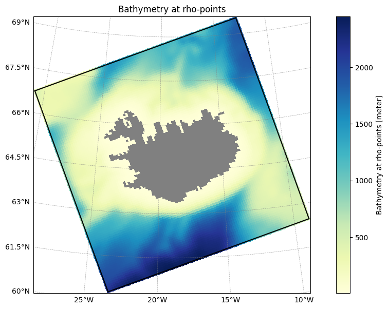
We can create a ROMS grid, mask, topography, and vertical coordinate system by creating an instance of the Grid class. In this example our grid spans the Nordic Seas and has a horizontal resolution of 10km and 100 vertical layers.
[2]:
%%time

grid = Grid(
    nx=250,  # number of grid points in x-direction
    ny=250,  # number of grid points in y-direction
    size_x=2500,  # domain size in x-direction (in km)
    size_y=2500,  # domain size in y-direction (in km)
    center_lon=-15,  # longitude of the center of the domain
    center_lat=65,  # latitude of the center of the domain
    rot=-30,  # rotation of the grid (in degrees)
    topography_source={
        "name": "SRTM15",
        "path": "/anvil/projects/x-ees250129/Datasets/SRTM15/SRTM15_V2.6.nc",
    },
    N=100,  # number of vertical layers
    verbose=True,
)
2026-04-01 13:21:11 - INFO - === Creating the horizontal grid ===
2026-04-01 13:21:11 - INFO - Total time: 0.099 seconds
2026-04-01 13:21:11 - INFO - ================================================================================================
2026-04-01 13:21:11 - INFO - === Making the mask ===
2026-04-01 13:21:12 - INFO - Inferring the mask from coastlines: 0.288 seconds
2026-04-01 13:21:12 - INFO - Filling enclosed basins with land: 0.007 seconds
2026-04-01 13:21:12 - INFO - Total time: 0.297 seconds
2026-04-01 13:21:12 - INFO - ================================================================================================
2026-04-01 13:21:12 - INFO - === Generating the topography using SRTM15 data and hmin = 5.0 meters ===
2026-04-01 13:21:12 - INFO - Reading the topography data: 0.147 seconds
2026-04-01 13:21:14 - INFO - Regridding the topography: 0.482 seconds
2026-04-01 13:21:14 - INFO - Domain-wide topography smoothing: 0.012 seconds
2026-04-01 13:21:17 - INFO - Local topography smoothing: 2.252 seconds
2026-04-01 13:21:17 - INFO - Total time: 4.748 seconds
2026-04-01 13:21:17 - INFO - ================================================================================================
2026-04-01 13:21:17 - INFO - === Preparing the vertical coordinate system using N = 100, theta_s = 5.0, theta_b = 2.0, hc = 300.0 ===
2026-04-01 13:21:17 - INFO - Total time: 0.003 seconds
2026-04-01 13:21:17 - INFO - ================================================================================================
CPU times: user 4.47 s, sys: 370 ms, total: 4.84 s
Wall time: 5.17 s
We generated the grid with verbose mode enabled, allowing us to see which steps were taken and how long each took. As you can see from the printed output, the four main steps are as follows:
We will explore steps II., III., and IV. in more detail later. For now, let’s examine the grid variables that were created, which can be found in the xarray.Dataset object returned by the .ds property.
[3]:
grid.ds
[3]:
<xarray.Dataset> Size: 7MB
Dimensions:       (eta_rho: 252, xi_rho: 252, xi_u: 251, eta_v: 251,
                   eta_coarse: 127, xi_coarse: 127, s_rho: 100, s_w: 101)
Coordinates:
    lat_rho       (eta_rho, xi_rho) float64 508kB 57.27 57.26 ... 64.56 64.48
    lon_rho       (eta_rho, xi_rho) float64 508kB 315.8 316.0 ... 22.61 22.7
    lat_u         (eta_rho, xi_u) float64 506kB 57.27 57.26 57.25 ... 64.6 64.52
    lon_u         (eta_rho, xi_u) float64 506kB 315.9 316.1 ... 22.56 22.66
    lat_v         (eta_v, xi_rho) float64 506kB 57.31 57.31 57.3 ... 64.54 64.46
    lon_v         (eta_v, xi_rho) float64 506kB 315.8 316.0 ... 22.52 22.61
    lat_coarse    (eta_coarse, xi_coarse) float64 129kB 57.23 57.22 ... 64.46
    lon_coarse    (eta_coarse, xi_coarse) float64 129kB 315.8 316.1 ... 22.84
Dimensions without coordinates: eta_rho, xi_rho, xi_u, eta_v, eta_coarse,
                                xi_coarse, s_rho, s_w
Data variables: (12/15)
    angle         (eta_rho, xi_rho) float64 508kB -0.05794 -0.05794 ... -1.102
    f             (eta_rho, xi_rho) float64 508kB 0.0001223 ... 0.0001313
    pm            (eta_rho, xi_rho) float64 508kB 0.0001019 ... 0.0001019
    pn            (eta_rho, xi_rho) float64 508kB 0.0001019 ... 0.0001019
    spherical     |S1 1B b'T'
    mask_rho      (eta_rho, xi_rho) int32 254kB 1 1 1 1 1 1 1 ... 0 0 0 0 0 0 0
    ...            ...
    mask_coarse   (eta_coarse, xi_coarse) int32 65kB 1 1 1 1 1 1 ... 0 0 0 0 0 0
    h             (eta_rho, xi_rho) float64 508kB 3.386e+03 3.386e+03 ... 71.21
    sigma_r       (s_rho) float32 400B -0.995 -0.985 -0.975 ... -0.015 -0.005
    Cs_r          (s_rho) float32 400B -0.992 -0.9753 ... -8.89e-05 -9.874e-06
    sigma_w       (s_w) float32 404B -1.0 -0.99 -0.98 -0.97 ... -0.02 -0.01 0.0
    Cs_w          (s_w) float32 404B -1.0 -0.9837 -0.9667 ... -3.95e-05 0.0
Attributes: (12/14)
    title:                   ROMS grid created by ROMS-Tools
    roms_tools_version:      3.4.1.dev23+g4c81e9a67
    size_x:                  2500
    size_y:                  2500
    center_lon:              -15
    center_lat:              65
    ...                      ...
    topography_source_name:  SRTM15
    topography_source_path:  /anvil/projects/x-ees250129/Datasets/SRTM15/SRTM...
    hmin:                    5.0
    theta_s:                 5.0
    theta_b:                 2.0
hc: 300.0Use the .plot() method to visualize the grid you just created, along with its bathymetry.
[4]:
grid.plot()

We can also plot the grid along a fixed latitude or longitude to examine its bathymetry in cross-section.
[5]:
grid.plot(lat=65)

[6]:
grid.plot(lon=-20)

Saving as NetCDF or YAML file#
Once we are happy with our grid, we can save it as a netCDF file via the .save method:
[7]:
filepath = "/anvil/projects/x-ees250129/x-uheede/grids/my_roms_grid.nc"
[8]:
grid.save(filepath)
2026-03-16 17:37:27 - INFO - Writing the following NetCDF files:
/anvil/projects/x-ees250129/x-uheede/grids/my_roms_grid.nc
[8]:
[PosixPath('/anvil/projects/x-ees250129/x-uheede/grids/my_roms_grid.nc')]
We can also export the grid parameters to a YAML file. This gives us a more storage-effective way to save and share input data made with ROMS-Tools. The YAML file can be used to recreate the same grid object later.
[9]:
yaml_filepath = "/anvil/projects/x-ees250129/x-uheede/grids/my_roms_grid.yaml"
[10]:
grid.to_yaml(yaml_filepath)
These are the contents of the written YAML file.
[11]:
# Open and read the YAML file
with open(yaml_filepath, "r") as file:
    file_contents = file.read()

# Print the contents
print(file_contents)
---
roms_tools_version: 3.4.1.dev23+g4c81e9a67
---
Grid:
  nx: 250
  ny: 250
  size_x: 2500
  size_y: 2500
  center_lon: -15
  center_lat: 65
  rot: -30
  N: 100
  theta_s: 5.0
  theta_b: 2.0
  hc: 300.0
  topography_source:
    name: SRTM15
    path: /anvil/projects/x-ees250129/Datasets/SRTM15/SRTM15_V2.6.nc
  mask_shapefile: null
  close_narrow_channels: false
  hmin: 5.0
Creating a grid from an existing NetCDF or YAML file#
We can also create a grid from an existing file.
[12]:
the_same_grid = Grid(filename=filepath)
[13]:
the_same_grid.ds
[13]:
<xarray.Dataset> Size: 7MB
Dimensions:       (eta_rho: 252, xi_rho: 252, xi_u: 251, eta_v: 251,
                   eta_coarse: 127, xi_coarse: 127, s_rho: 100, s_w: 101)
Coordinates:
    lat_rho       (eta_rho, xi_rho) float64 508kB ...
    lon_rho       (eta_rho, xi_rho) float64 508kB ...
    lat_u         (eta_rho, xi_u) float64 506kB ...
    lon_u         (eta_rho, xi_u) float64 506kB ...
    lat_v         (eta_v, xi_rho) float64 506kB ...
    lon_v         (eta_v, xi_rho) float64 506kB ...
    lat_coarse    (eta_coarse, xi_coarse) float64 129kB ...
    lon_coarse    (eta_coarse, xi_coarse) float64 129kB ...
Dimensions without coordinates: eta_rho, xi_rho, xi_u, eta_v, eta_coarse,
                                xi_coarse, s_rho, s_w
Data variables: (12/15)
    angle         (eta_rho, xi_rho) float64 508kB ...
    f             (eta_rho, xi_rho) float64 508kB ...
    pm            (eta_rho, xi_rho) float64 508kB ...
    pn            (eta_rho, xi_rho) float64 508kB ...
    spherical     |S1 1B ...
    mask_rho      (eta_rho, xi_rho) int32 254kB ...
    ...            ...
    mask_coarse   (eta_coarse, xi_coarse) int32 65kB ...
    h             (eta_rho, xi_rho) float64 508kB ...
    sigma_r       (s_rho) float32 400B ...
    Cs_r          (s_rho) float32 400B ...
    sigma_w       (s_w) float32 404B ...
    Cs_w          (s_w) float32 404B ...
Attributes: (12/14)
    title:                   ROMS grid created by ROMS-Tools
    roms_tools_version:      3.4.1.dev23+g4c81e9a67
    size_x:                  2500
    size_y:                  2500
    center_lon:              -15
    center_lat:              65
    ...                      ...
    topography_source_name:  SRTM15
    topography_source_path:  /anvil/projects/x-ees250129/Datasets/SRTM15/SRTM...
    hmin:                    5.0
    theta_s:                 5.0
    theta_b:                 2.0
hc: 300.0Alternatively, we can create a grid from an existing YAML file.
[14]:
%time yet_the_same_grid = Grid.from_yaml(yaml_filepath, verbose=False)
CPU times: user 4.42 s, sys: 359 ms, total: 4.78 s
Wall time: 4.76 s
[15]:
yet_the_same_grid.ds
[15]:
<xarray.Dataset> Size: 7MB
Dimensions:       (eta_rho: 252, xi_rho: 252, xi_u: 251, eta_v: 251,
                   eta_coarse: 127, xi_coarse: 127, s_rho: 100, s_w: 101)
Coordinates:
    lat_rho       (eta_rho, xi_rho) float64 508kB 57.27 57.26 ... 64.56 64.48
    lon_rho       (eta_rho, xi_rho) float64 508kB 315.8 316.0 ... 22.61 22.7
    lat_u         (eta_rho, xi_u) float64 506kB 57.27 57.26 57.25 ... 64.6 64.52
    lon_u         (eta_rho, xi_u) float64 506kB 315.9 316.1 ... 22.56 22.66
    lat_v         (eta_v, xi_rho) float64 506kB 57.31 57.31 57.3 ... 64.54 64.46
    lon_v         (eta_v, xi_rho) float64 506kB 315.8 316.0 ... 22.52 22.61
    lat_coarse    (eta_coarse, xi_coarse) float64 129kB 57.23 57.22 ... 64.46
    lon_coarse    (eta_coarse, xi_coarse) float64 129kB 315.8 316.1 ... 22.84
Dimensions without coordinates: eta_rho, xi_rho, xi_u, eta_v, eta_coarse,
                                xi_coarse, s_rho, s_w
Data variables: (12/15)
    angle         (eta_rho, xi_rho) float64 508kB -0.05794 -0.05794 ... -1.102
    f             (eta_rho, xi_rho) float64 508kB 0.0001223 ... 0.0001313
    pm            (eta_rho, xi_rho) float64 508kB 0.0001019 ... 0.0001019
    pn            (eta_rho, xi_rho) float64 508kB 0.0001019 ... 0.0001019
    spherical     |S1 1B b'T'
    mask_rho      (eta_rho, xi_rho) int32 254kB 1 1 1 1 1 1 1 ... 0 0 0 0 0 0 0
    ...            ...
    mask_coarse   (eta_coarse, xi_coarse) int32 65kB 1 1 1 1 1 1 ... 0 0 0 0 0 0
    h             (eta_rho, xi_rho) float64 508kB 3.386e+03 3.386e+03 ... 71.21
    sigma_r       (s_rho) float32 400B -0.995 -0.985 -0.975 ... -0.015 -0.005
    Cs_r          (s_rho) float32 400B -0.992 -0.9753 ... -8.89e-05 -9.874e-06
    sigma_w       (s_w) float32 404B -1.0 -0.99 -0.98 -0.97 ... -0.02 -0.01 0.0
    Cs_w          (s_w) float32 404B -1.0 -0.9837 -0.9667 ... -3.95e-05 0.0
Attributes: (12/14)
    title:                   ROMS grid created by ROMS-Tools
    roms_tools_version:      3.4.1.dev23+g4c81e9a67
    size_x:                  2500
    size_y:                  2500
    center_lon:              -15
    center_lat:              65
    ...                      ...
    topography_source_name:  SRTM15
    topography_source_path:  /anvil/projects/x-ees250129/Datasets/SRTM15/SRTM...
    hmin:                    5.0
    theta_s:                 5.0
    theta_b:                 2.0
hc: 300.0Mask#
The land–sea mask is generated by comparing the grid’s latitude and longitude coordinates with a coastline dataset provided as a shapefile.
Mask Shapefile#
The coastline dataset is supplied through the mask_shapefile parameter when creating the grid object.
If no shapefile is provided, ROMS-Tools automatically falls back to the Natural Earth 1:10m coastline dataset (used in the example above). The label 1:10m refers to a map scale of 1:10,000,000, which corresponds to an effective spatial resolution of approximately 1–5 km.
To improve the accuracy of the land–sea mask, especially for fjords, narrow straits, and other complex coastal geometries, we next explore several resolutions of the GSHHG coastline dataset.
GSHHG provides five resolutions:
f (full): original highest-detail dataset
h (high): ~80% reduction in detail and file size
i (intermediate): another ~80% reduction
l (low): another ~80% reduction
c (crude): another ~80% reduction
Higher-resolution versions offer more accurate coastlines but require substantially more memory when generating the mask. In the following, we therefore profile the memory usage.
[3]:
%load_ext memory_profiler
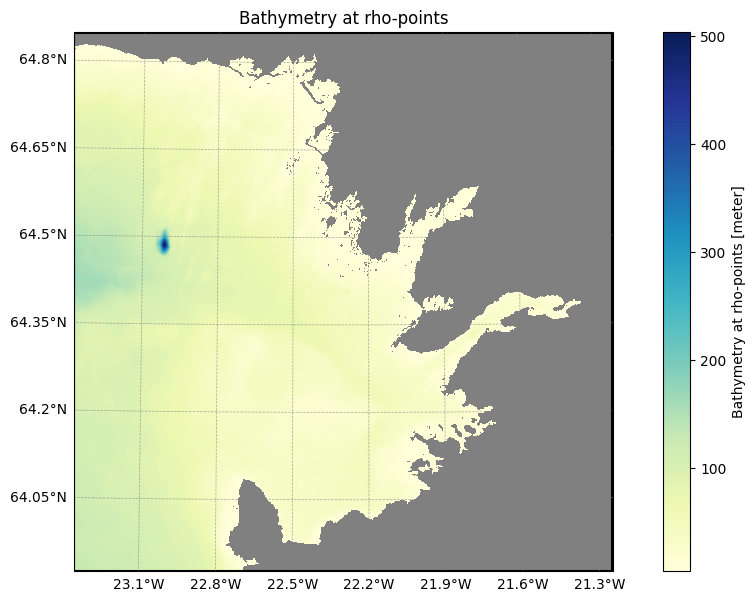
We will compare the masks derived from Natural Earth and GSHHG for a ROMS grid representing Hvalfjörður fjord in Iceland at 50 m horizontal resolution.
[4]:
iceland_fjord_kwargs = {
    "nx": 800,
    "ny": 400,
    "size_x": 40,
    "size_y": 20,
    "center_lon": -21.76,
    "center_lat": 64.325,
    "rot": 0,
    "topography_source": {
        "name": "SRTM15",
        "path": "/anvil/projects/x-ees250129/Datasets/SRTM15/SRTM15_V2.6.nc"
    },
    "N": 40
}
First, we create a land-sea mask using the default Natural Earth coastline (i.e., withouth specifying a mask_shapefile).
[5]:
%%time
%%memit

fjord_grid_natural_earth = Grid(**iceland_fjord_kwargs, verbose=True)
2026-04-01 13:22:00 - INFO - === Creating the horizontal grid ===
2026-04-01 13:22:00 - INFO - Total time: 0.421 seconds
2026-04-01 13:22:00 - INFO - ================================================================================================
2026-04-01 13:22:00 - INFO - === Making the mask ===
2026-04-01 13:22:01 - INFO - Inferring the mask from coastlines: 0.413 seconds
2026-04-01 13:22:01 - INFO - Filling enclosed basins with land: 0.002 seconds
2026-04-01 13:22:01 - INFO - Total time: 0.417 seconds
2026-04-01 13:22:01 - INFO - ================================================================================================
2026-04-01 13:22:01 - INFO - === Generating the topography using SRTM15 data and hmin = 5.0 meters ===
2026-04-01 13:22:01 - INFO - Reading the topography data: 0.013 seconds
2026-04-01 13:22:01 - INFO - Regridding the topography: 0.015 seconds
2026-04-01 13:22:01 - INFO - Domain-wide topography smoothing: 0.029 seconds
2026-04-01 13:22:02 - INFO - Local topography smoothing: 0.739 seconds
2026-04-01 13:22:02 - INFO - Total time: 0.809 seconds
2026-04-01 13:22:02 - INFO - ================================================================================================
2026-04-01 13:22:02 - INFO - === Preparing the vertical coordinate system using N = 40, theta_s = 5.0, theta_b = 2.0, hc = 300.0 ===
2026-04-01 13:22:02 - INFO - Total time: 0.003 seconds
2026-04-01 13:22:02 - INFO - ================================================================================================
peak memory: 705.34 MiB, increment: 89.58 MiB
CPU times: user 1.72 s, sys: 121 ms, total: 1.84 s
Wall time: 1.94 s
Mask creation was very fast (< 1 second), and the total memory footprint of the grid generation was small (< 1 GB). However, the next plot shows that the Natural Earth coastline provides only a coarse representation of Hvalfjörður, resulting in an overly smooth and poorly resolved shoreline.
[6]:
fjord_grid_natural_earth.plot()

Next, we explore the high-resolution (h) version of the GSHHG dataset to generate the land–sea mask.
[7]:
%%time
%%memit

fjord_grid_gshhg_h = Grid(
    **iceland_fjord_kwargs,
    mask_shapefile="/anvil/projects/x-ees250129/Datasets/GSHHS/gshhg-shp-2.3.7/GSHHS_shp/h/GSHHS_h_L1.shp",
    verbose=True
)
2026-04-01 13:22:12 - INFO - === Creating the horizontal grid ===
2026-04-01 13:22:12 - INFO - Total time: 0.434 seconds
2026-04-01 13:22:12 - INFO - ================================================================================================
2026-04-01 13:22:12 - INFO - === Making the mask ===
2026-04-01 13:22:28 - INFO - Inferring the mask from coastlines: 15.794 seconds
2026-04-01 13:22:28 - INFO - Filling enclosed basins with land: 0.003 seconds
2026-04-01 13:22:28 - INFO - Total time: 15.842 seconds
2026-04-01 13:22:28 - INFO - ================================================================================================
2026-04-01 13:22:28 - INFO - === Generating the topography using SRTM15 data and hmin = 5.0 meters ===
2026-04-01 13:22:28 - INFO - Reading the topography data: 0.015 seconds
2026-04-01 13:22:28 - INFO - Regridding the topography: 0.015 seconds
2026-04-01 13:22:28 - INFO - Domain-wide topography smoothing: 0.034 seconds
2026-04-01 13:22:29 - INFO - Local topography smoothing: 0.752 seconds
2026-04-01 13:22:29 - INFO - Total time: 0.828 seconds
2026-04-01 13:22:29 - INFO - ================================================================================================
2026-04-01 13:22:29 - INFO - === Preparing the vertical coordinate system using N = 40, theta_s = 5.0, theta_b = 2.0, hc = 300.0 ===
2026-04-01 13:22:29 - INFO - Total time: 0.003 seconds
2026-04-01 13:22:29 - INFO - ================================================================================================
peak memory: 45282.23 MiB, increment: 44587.82 MiB
CPU times: user 13.4 s, sys: 3.62 s, total: 17.1 s
Wall time: 17.4 s
Creating the mask now took about 15 seconds, and the overall memory footprint of the grid increased to roughly 45 GB: relatively high. The coastlines are better resolved than with Natural Earth, though still somewhat angular due to the data reduction applied in this GSHHG resolution.
[21]:
fjord_grid_gshhg_h.plot()

Finally, we use the full-resolution GSHHG dataset to generate the land–sea mask.
[8]:
%%time
%%memit

fjord_grid_gshhg_f = Grid(
    **iceland_fjord_kwargs,
    mask_shapefile="/anvil/projects/x-ees250129/Datasets/GSHHS/gshhg-shp-2.3.7/GSHHS_shp/f/GSHHS_f_L1.shp",
    verbose=True
)
2026-04-01 13:22:37 - INFO - === Creating the horizontal grid ===
2026-04-01 13:22:37 - INFO - Total time: 0.437 seconds
2026-04-01 13:22:37 - INFO - ================================================================================================
2026-04-01 13:22:37 - INFO - === Making the mask ===
2026-04-01 13:22:57 - INFO - Inferring the mask from coastlines: 19.963 seconds
2026-04-01 13:22:57 - INFO - Filling enclosed basins with land: 0.002 seconds
2026-04-01 13:22:57 - INFO - Total time: 20.017 seconds
2026-04-01 13:22:57 - INFO - ================================================================================================
2026-04-01 13:22:57 - INFO - === Generating the topography using SRTM15 data and hmin = 5.0 meters ===
2026-04-01 13:22:57 - INFO - Reading the topography data: 0.018 seconds
2026-04-01 13:22:57 - INFO - Regridding the topography: 0.015 seconds
2026-04-01 13:22:57 - INFO - Domain-wide topography smoothing: 0.031 seconds
2026-04-01 13:22:58 - INFO - Local topography smoothing: 0.765 seconds
2026-04-01 13:22:58 - INFO - Total time: 0.842 seconds
2026-04-01 13:22:58 - INFO - ================================================================================================
2026-04-01 13:22:58 - INFO - === Preparing the vertical coordinate system using N = 40, theta_s = 5.0, theta_b = 2.0, hc = 300.0 ===
2026-04-01 13:22:58 - INFO - Total time: 0.003 seconds
2026-04-01 13:22:58 - INFO - ================================================================================================
peak memory: 56353.35 MiB, increment: 55625.62 MiB
CPU times: user 16.7 s, sys: 4.55 s, total: 21.2 s
Wall time: 21.6 s
Creating the mask now took about 20 seconds, and the grid’s memory footprint increased to roughly 55 GB: even higher. However, the coastline is captured in much greater detail using the full-resolution GSHHG data.
[23]:
fjord_grid_gshhg_f.plot()

Note
For very large grids with many points, using the full-resolution GSHHG dataset may exceed available memory. You may need to experiment to find the optimal coastline resolution. For most applications, the Natural Earth coastlines may provide a sufficiently accurate representation.
Closing narrow channels#
When creating a grid, you have the option to set close_narrow_channels to True. This functionality cleans up the land-sea mask by removing narrow 1-pixel wide passages. This is particularly useful when working with high-resolution coastline datasets that may create unrealistic narrow channels that could cause instabilities in ROMS.
The method performs one main operation:
Closes narrow 1-pixel channels: Iteratively removes 1-pixel wide land passages in both north-south and east-west directions. After closing, the velocity masks (mask_u and mask_v) are automatically updated to reflect the changes in mask_rho and any lakes/holes in the mask generated by closing narrow passages are filled subsequently.
Let’s create two grids and look at the difference to demonstrate the functionality. We’ll use a grid with a relatively high resolution to show how narrow passages can be problematic.
[9]:
# Create a fine-scale grid for demonstration

# Create common grid kwargs for both grids
kwargs = {
    "nx": 512,
    "ny": 512,
    "size_x": 102.4,
    "size_y": 102.4,
    "center_lon": -22.3,
    "center_lat": 64.39,
    "rot": 0,
    "mask_shapefile": "/anvil/projects/x-ees250129/Datasets/GSHHS/gshhg-shp-2.3.7/GSHHS_shp/f/GSHHS_f_L1.shp",
    "topography_source" :{
        "name": "EMOD",
        "path": "/anvil/projects/x-ees250129/Datasets/EMODnet_C2.nc"
    },
    "N": 60, # number of vertical layers
    "verbose": True
}

# Set close_narrow_channels to False
narrow_channel_false_grid = Grid(
    **kwargs,
    close_narrow_channels=False # this is the default
)

# Set close_narrow_channels to True
narrow_channel_true_grid = Grid(
    **kwargs,
    close_narrow_channels=True
)

# Plot without closed channels
narrow_channel_false_grid.plot()
2026-04-01 13:23:16 - INFO - === Creating the horizontal grid ===
2026-04-01 13:23:16 - INFO - Total time: 0.326 seconds
2026-04-01 13:23:16 - INFO - ================================================================================================
2026-04-01 13:23:16 - INFO - === Making the mask ===
2026-04-01 13:23:31 - INFO - Inferring the mask from coastlines: 14.484 seconds
2026-04-01 13:23:31 - INFO - Filling enclosed basins with land: 0.011 seconds
2026-04-01 13:23:31 - INFO - Total time: 14.543 seconds
2026-04-01 13:23:31 - INFO - ================================================================================================
2026-04-01 13:23:31 - INFO - === Generating the topography using EMOD data and hmin = 5.0 meters ===
2026-04-01 13:23:32 - INFO - Reading the topography data: 1.111 seconds
2026-04-01 13:23:38 - INFO - Regridding the topography: 0.027 seconds
2026-04-01 13:23:38 - INFO - Domain-wide topography smoothing: 0.027 seconds
2026-04-01 13:23:39 - INFO - Local topography smoothing: 0.345 seconds
2026-04-01 13:23:39 - INFO - Total time: 7.893 seconds
2026-04-01 13:23:39 - INFO - ================================================================================================
2026-04-01 13:23:39 - INFO - === Preparing the vertical coordinate system using N = 60, theta_s = 5.0, theta_b = 2.0, hc = 300.0 ===
2026-04-01 13:23:39 - INFO - Total time: 0.003 seconds
2026-04-01 13:23:39 - INFO - ================================================================================================
2026-04-01 13:23:39 - INFO - === Creating the horizontal grid ===
2026-04-01 13:23:39 - INFO - Total time: 0.321 seconds
2026-04-01 13:23:39 - INFO - ================================================================================================
2026-04-01 13:23:39 - INFO - === Making the mask ===
2026-04-01 13:23:53 - INFO - Inferring the mask from coastlines: 14.352 seconds
2026-04-01 13:23:53 - INFO - Closing narrow channels: 0.024 seconds
2026-04-01 13:23:53 - INFO - Filling enclosed basins with land: 0.005 seconds
2026-04-01 13:23:53 - INFO - Total time: 14.435 seconds
2026-04-01 13:23:53 - INFO - ================================================================================================
2026-04-01 13:23:53 - INFO - === Generating the topography using EMOD data and hmin = 5.0 meters ===
2026-04-01 13:23:54 - INFO - Reading the topography data: 0.360 seconds
2026-04-01 13:24:00 - INFO - Regridding the topography: 0.028 seconds
2026-04-01 13:24:00 - INFO - Domain-wide topography smoothing: 0.027 seconds
2026-04-01 13:24:00 - INFO - Local topography smoothing: 0.347 seconds
2026-04-01 13:24:00 - INFO - Total time: 6.533 seconds
2026-04-01 13:24:00 - INFO - ================================================================================================
2026-04-01 13:24:00 - INFO - === Preparing the vertical coordinate system using N = 60, theta_s = 5.0, theta_b = 2.0, hc = 300.0 ===
2026-04-01 13:24:00 - INFO - Total time: 0.003 seconds
2026-04-01 13:24:00 - INFO - ================================================================================================
Now, let’s look at the difference between the two plots.
[10]:
from roms_tools.plot import plot

# Plot the difference (areas that were changed)
mask_diff = narrow_channel_false_grid.ds.mask_rho - narrow_channel_true_grid.ds.mask_rho
plot(mask_diff, grid_ds=narrow_channel_true_grid.ds, apply_mask=False)

The plot above shows where the mask was modified. Red areas indicate where water was converted to land.
Updating the mask#
If you want to update the land–sea mask while keeping the existing horizontal grid, topography, and vertical coordinate system, you can skip Steps I, III, and IV. This can be easily done using the .update_mask method.
Here, we update the grid created at the beginning of this notebook (using the Natural Earth coastlines) with a mask derived from the GSHHG dataset.
[ ]:
%%time
%%memit

grid.update_mask(
    mask_shapefile="/anvil/projects/x-ees250129/Datasets/GSHHS/gshhg-shp-2.3.7/GSHHS_shp/f/GSHHS_f_L1.shp",
    close_narrow_channels=True,
    verbose=True
  )
The new shapefile is now also recorded in the grid attributes.
[11]:
grid
[11]:
Grid(nx=250, ny=250, size_x=2500, size_y=2500, center_lon=-15, center_lat=65, rot=-30, N=100, theta_s=5.0, theta_b=2.0, hc=300.0, topography_source={'name': 'SRTM15', 'path': '/anvil/projects/x-ees250129/Datasets/SRTM15/SRTM15_V2.6.nc'}, close_narrow_channels=False, hmin=5.0, verbose=True, straddle=True)
[12]:
grid.plot()

Let’s save a copy of the mask before updating the grid again to switch back to the Natural Earth–derived mask.
[29]:
nordic_mask_gshhg = grid.ds.mask_rho.copy()
We now switch back to the Natural Earth–derived mask.
[30]:
grid.update_mask(
    verbose=True
)
2026-02-08 11:59:51 - INFO - === Deriving the mask from coastlines ===
2026-02-08 11:59:51 - INFO - Total time: 0.196 seconds
2026-02-08 11:59:51 - INFO - ================================================================================================
[31]:
grid
[31]:
Grid(nx=250, ny=250, size_x=2500, size_y=2500, center_lon=-15, center_lat=65, rot=-30, N=100, theta_s=5.0, theta_b=2.0, hc=300.0, topography_source={'name': 'SRTM15', 'path': '/anvil/projects/x-ees250129/Datasets/SRTM15/SRTM15_V2.6.nc'}, close_narrow_channels=False, hmin=5.0, verbose=True, straddle=True)
[32]:
nordic_mask_natural_earth = grid.ds.mask_rho.copy()
The next plot shows the difference between the two masks.
[33]:
from roms_tools.plot import plot
plot(nordic_mask_gshhg - nordic_mask_natural_earth, grid_ds=grid.ds, apply_mask=False)

The red and yellow dots along the coastline show where the two coastline datasets produce different land-sea masks and where narrow channels were closed.
Topography#
Here you can find an overview of the steps involved in the topography generation. In the following, we will illustrate how these concepts work in practice.
Topography source data#
The grid object includes a parameter called topography_source. If this parameter is not specified, it defaults to using the ETOPO5 topography data. The ETOPO5 data is downloaded internally, so the user does not need to provide a filename.
The ETOPO5 data has a horizontal resolution of 5 arc-minutes (or 1/12th of a degree). This horizontal resolution may be sufficient for coarser-resolution grids, but for finer-resolution grids we might want to use the finer-resolution topography product SRTM15. SRTM15 has a horizontal resolution of 15 arc-seconds (or 1/240th of a degree).
Let’s compare the topographies that are generated from ETOPO5 versus SRTM15 data for a ROMS grid surrounding Iceland.
[34]:
iceland_kwargs = {
    "size_x": 800,
    "size_y": 800,
    "center_lon": -19,
    "center_lat": 65,
    "rot": 20,
}
First, we generate two “coarse-resolution” grids with a horizontal resolution of 800km/100 = 8km: one regridded from the ETOPO5 data and the other from the SRTM15 data.
[35]:
%%time

coarse_grid_ETOPO5 = Grid(nx=100, ny=100, **iceland_kwargs, verbose=False)
CPU times: user 1.36 s, sys: 9.94 ms, total: 1.37 s
Wall time: 1.38 s
[36]:
%%time

coarse_grid_SRTM15 = Grid(
    nx=100,
    ny=100,
    topography_source={
        "name": "SRTM15",
        "path": "/anvil/projects/x-ees250129/Datasets/SRTM15/SRTM15_V2.6.nc",
    },
    **iceland_kwargs,
    verbose=False
)
CPU times: user 1.58 s, sys: 46.8 ms, total: 1.62 s
Wall time: 1.63 s
Comparing the timings above, we can see that generating the topographies took a similar amount of time and was quick overall. Next, let’s compare the generated topography fields.
[37]:
coarse_grid_ETOPO5.plot()

[38]:
coarse_grid_SRTM15.plot()
Comparing the figures above, we don’t see significant differences in the generated topography fields. The grid is simply too coarse to fully utilize the high-resolution SRTM15 data! To observe more noticeable differences, we need to use a finer resolution grid.
Let’s do that! Next, we generate two fine-resolution grids with a horizontal resolution of 800km/5000 = 0.16km: one regridded from the ETOPO5 data and the other from the SRTM15 data.
[39]:
%%time

fine_grid = Grid(nx=5000, ny=5000, **iceland_kwargs, verbose=True)
2026-02-08 11:59:56 - INFO - === Creating the horizontal grid ===
2026-02-08 12:00:32 - INFO - Total time: 36.619 seconds
2026-02-08 12:00:32 - INFO - ================================================================================================
2026-02-08 12:00:33 - INFO - === Deriving the mask from coastlines ===
2026-02-08 12:01:05 - INFO - Total time: 32.618 seconds
2026-02-08 12:01:05 - INFO - ================================================================================================
2026-02-08 12:01:06 - INFO - === Generating the topography using ETOPO5 data and hmin = 5.0 meters ===
2026-02-08 12:01:06 - INFO - Reading the topography data: 0.026 seconds
2026-02-08 12:01:07 - INFO - Regridding the topography: 0.861 seconds
2026-02-08 12:01:11 - INFO - Domain-wide topography smoothing: 4.141 seconds
2026-02-08 12:02:32 - INFO - Local topography smoothing: 80.996 seconds
2026-02-08 12:02:32 - INFO - Total time: 86.150 seconds
2026-02-08 12:02:32 - INFO - ================================================================================================
2026-02-08 12:02:32 - INFO - === Preparing the vertical coordinate system using N = 100, theta_s = 5.0, theta_b = 2.0, hc = 300.0 ===
2026-02-08 12:02:32 - INFO - Total time: 0.003 seconds
2026-02-08 12:02:32 - INFO - ================================================================================================
CPU times: user 2min 13s, sys: 21.9 s, total: 2min 35s
Wall time: 2min 36s
[40]:
%%time

fine_grid_SRTM15 = Grid(
    nx=5000,
    ny=5000,
    topography_source={
        "name": "SRTM15",
        "path": "/anvil/projects/x-ees250129/Datasets/SRTM15/SRTM15_V2.6.nc",
    },
    **iceland_kwargs,
    verbose=True
)
2026-02-08 12:02:32 - INFO - === Creating the horizontal grid ===
2026-02-08 12:03:07 - INFO - Total time: 35.193 seconds
2026-02-08 12:03:07 - INFO - ================================================================================================
2026-02-08 12:03:07 - INFO - === Deriving the mask from coastlines ===
2026-02-08 12:03:40 - INFO - Total time: 32.596 seconds
2026-02-08 12:03:40 - INFO - ================================================================================================
2026-02-08 12:03:41 - INFO - === Generating the topography using SRTM15 data and hmin = 5.0 meters ===
2026-02-08 12:03:41 - INFO - Reading the topography data: 0.012 seconds
2026-02-08 12:03:42 - INFO - Regridding the topography: 1.384 seconds
2026-02-08 12:03:47 - INFO - Domain-wide topography smoothing: 4.398 seconds
2026-02-08 12:05:25 - INFO - Local topography smoothing: 97.790 seconds
2026-02-08 12:05:25 - INFO - Total time: 103.867 seconds
2026-02-08 12:05:25 - INFO - ================================================================================================
2026-02-08 12:05:25 - INFO - === Preparing the vertical coordinate system using N = 100, theta_s = 5.0, theta_b = 2.0, hc = 300.0 ===
2026-02-08 12:05:25 - INFO - Total time: 0.003 seconds
2026-02-08 12:05:25 - INFO - ================================================================================================
CPU times: user 2min 33s, sys: 18 s, total: 2min 51s
Wall time: 2min 52s
The grid and topography generation process took longer this time, but the durations for both cases were quite similar.
Note that most of the time was spent during the local smoothing phase in both cases. The goal of this smoothing is to ensure that the local steepness ratio does not exceed the threshold of 0.2. Because the topography data contains a lot of details for such a fine-resolution grid, the local smoothing required many iterations for smoothing.
Let’s take a look at the generated topography fields.
[41]:
fine_grid.plot() # grid with ETOPO5 topography

[42]:
fine_grid_SRTM15.plot() # grid with SRTM15 topography

The two figures above reveal differences: the topography generated with the SRTM15 data shows a lot more detail. If we moved to an even finer resolution, these differences would become even more pronounced.
The minimal ocean depth hmin#
The default for hmin is 5 meters. In the above examples, we did not specify the (optional) hmin parameter, so it was set to the default value.
[43]:
fine_grid.hmin
[43]:
5.0
Let’s confirm that the minimum ocean depth is indeed at least 5 meters.
[44]:
fine_grid.ds["h"].min()
[44]:
<xarray.DataArray 'h' ()> Size: 8B
array(5.)
We can define a grid with a different hmin.
[45]:
%%time

fine_grid_with_larger_hmin = Grid(
    nx=5000,
    ny=5000,
    **iceland_kwargs,
    verbose=True,
    hmin=10.0,  # Minimum ocean depth in meters (default: 5.0)
)
2026-02-08 12:06:35 - INFO - === Creating the horizontal grid ===
2026-02-08 12:07:12 - INFO - Total time: 36.270 seconds
2026-02-08 12:07:12 - INFO - ================================================================================================
2026-02-08 12:07:12 - INFO - === Deriving the mask from coastlines ===
2026-02-08 12:07:45 - INFO - Total time: 33.180 seconds
2026-02-08 12:07:45 - INFO - ================================================================================================
2026-02-08 12:07:46 - INFO - === Generating the topography using ETOPO5 data and hmin = 10.0 meters ===
2026-02-08 12:07:46 - INFO - Reading the topography data: 0.026 seconds
2026-02-08 12:07:47 - INFO - Regridding the topography: 0.865 seconds
2026-02-08 12:07:51 - INFO - Domain-wide topography smoothing: 4.311 seconds
2026-02-08 12:08:30 - INFO - Local topography smoothing: 38.933 seconds
2026-02-08 12:08:30 - INFO - Total time: 44.240 seconds
2026-02-08 12:08:30 - INFO - ================================================================================================
2026-02-08 12:08:30 - INFO - === Preparing the vertical coordinate system using N = 100, theta_s = 5.0, theta_b = 2.0, hc = 300.0 ===
2026-02-08 12:08:30 - INFO - Total time: 0.003 seconds
2026-02-08 12:08:30 - INFO - ================================================================================================
CPU times: user 1min 40s, sys: 13.3 s, total: 1min 54s
Wall time: 1min 54s
[46]:
fine_grid_with_larger_hmin.ds["h"].min()
[46]:
<xarray.DataArray 'h' ()> Size: 8B
array(10.)
Updating topography and hmin#
When working with a grid that has a large number of grid points, such as nx = ny = 5000 in the example above, Steps I and II (creating the horizontal grid and land mask) can be quite time-consuming: it took about 40 + 30 = 70 seconds! If you simply want to repeat Step III, which involves updating the topography and/or hmin, but you would like to keep the same horizontal grid and mask, you can skip Steps I, II, and IV. This can be easily achieved using the .update_topography
method. In the next cell, we take our fine resolution grid with ETOPO5 topography, and update it with SRTM15 topography and a larger hmin of 10 meters.
[47]:
%%time

fine_grid.update_topography(
    hmin=10.0,
    topography_source={
        "name": "SRTM15",
        "path": "/anvil/projects/x-ees250129/Datasets/SRTM15/SRTM15_V2.6.nc",
    },
    verbose=True,
)
2026-02-08 12:08:30 - INFO - === Generating the topography using SRTM15 data and hmin = 10.0 meters ===
2026-02-08 12:08:30 - INFO - Reading the topography data: 0.020 seconds
2026-02-08 12:08:32 - INFO - Regridding the topography: 1.412 seconds
2026-02-08 12:08:36 - INFO - Domain-wide topography smoothing: 4.301 seconds
2026-02-08 12:09:35 - INFO - Local topography smoothing: 58.472 seconds
2026-02-08 12:09:35 - INFO - Total time: 64.526 seconds
2026-02-08 12:09:35 - INFO - ================================================================================================
CPU times: user 53.2 s, sys: 11.2 s, total: 1min 4s
Wall time: 1min 4s
From the printed output, you can see that Steps I, II, and IV were skipped as desired. The following confirms that the topography_source and hmin were indeed updated.
[48]:
fine_grid
[48]:
Grid(nx=5000, ny=5000, size_x=800, size_y=800, center_lon=-19, center_lat=65, rot=20, N=100, theta_s=5.0, theta_b=2.0, hc=300.0, topography_source={'name': 'SRTM15', 'path': '/anvil/projects/x-ees250129/Datasets/SRTM15/SRTM15_V2.6.nc'}, close_narrow_channels=False, hmin=10.0, verbose=True, straddle=False)
The vertical coordinate system#
Here you can find an overview of the steps involved in creating the vertical coordinate system.
To prepare the vertical coordinate system, ROMS-Tools needs the following parameters:
N: the number of vertical layers (default: 100)theta_s: the surface control parameter (default: 5.0)theta_b: the bottom control parameter (default: 2.0)hc: the critical depth in meters (default: 300.0)
In the above examples, we did not specify the last three parameters, so they were set to the default values.
[49]:
grid
[49]:
Grid(nx=250, ny=250, size_x=2500, size_y=2500, center_lon=-15, center_lat=65, rot=-30, N=100, theta_s=5.0, theta_b=2.0, hc=300.0, topography_source={'name': 'SRTM15', 'path': '/anvil/projects/x-ees250129/Datasets/SRTM15/SRTM15_V2.6.nc'}, close_narrow_channels=False, hmin=5.0, verbose=True, straddle=True)
[50]:
print(f"N: {grid.N}, theta_s: {grid.theta_s}, theta_b: {grid.theta_b}, hc: {grid.hc}")
N: 100, theta_s: 5.0, theta_b: 2.0, hc: 300.0
Among the steps involved in generating the vertical coordinate system, only the first two are executed during grid generation. Specifically, the grid.ds object contains the vertical stretched coordinates (sigma_r and sigma_w), as well as the vertical stretching functions (Cs_r and Cs_w).
[51]:
grid.ds
[51]:
<xarray.Dataset> Size: 7MB
Dimensions:       (eta_rho: 252, xi_rho: 252, xi_u: 251, eta_v: 251,
                   eta_coarse: 127, xi_coarse: 127, s_rho: 100, s_w: 101)
Coordinates:
    lat_rho       (eta_rho, xi_rho) float64 508kB 57.27 57.26 ... 64.56 64.48
    lon_rho       (eta_rho, xi_rho) float64 508kB 315.8 316.0 ... 22.61 22.7
    lat_u         (eta_rho, xi_u) float64 506kB 57.27 57.26 57.25 ... 64.6 64.52
    lon_u         (eta_rho, xi_u) float64 506kB 315.9 316.1 ... 22.56 22.66
    lat_v         (eta_v, xi_rho) float64 506kB 57.31 57.31 57.3 ... 64.54 64.46
    lon_v         (eta_v, xi_rho) float64 506kB 315.8 316.0 ... 22.52 22.61
    lat_coarse    (eta_coarse, xi_coarse) float64 129kB 57.23 57.22 ... 64.46
    lon_coarse    (eta_coarse, xi_coarse) float64 129kB 315.8 316.1 ... 22.84
Dimensions without coordinates: eta_rho, xi_rho, xi_u, eta_v, eta_coarse,
                                xi_coarse, s_rho, s_w
Data variables: (12/15)
    angle         (eta_rho, xi_rho) float64 508kB -0.05794 -0.05794 ... -1.102
    f             (eta_rho, xi_rho) float64 508kB 0.0001223 ... 0.0001313
    pm            (eta_rho, xi_rho) float64 508kB 0.0001019 ... 0.0001019
    pn            (eta_rho, xi_rho) float64 508kB 0.0001019 ... 0.0001019
    spherical     |S1 1B b'T'
    mask_rho      (eta_rho, xi_rho) int32 254kB 1 1 1 1 1 1 1 ... 0 0 0 0 0 0 0
    ...            ...
    mask_coarse   (eta_coarse, xi_coarse) int32 65kB 1 1 1 1 1 1 ... 0 0 0 0 0 0
    h             (eta_rho, xi_rho) float64 508kB 3.386e+03 3.386e+03 ... 71.21
    sigma_r       (s_rho) float32 400B -0.995 -0.985 -0.975 ... -0.015 -0.005
    Cs_r          (s_rho) float32 400B -0.992 -0.9753 ... -8.89e-05 -9.874e-06
    sigma_w       (s_w) float32 404B -1.0 -0.99 -0.98 -0.97 ... -0.02 -0.01 0.0
    Cs_w          (s_w) float32 404B -1.0 -0.9837 -0.9667 ... -3.95e-05 0.0
Attributes: (12/15)
    title:                   ROMS grid created by ROMS-Tools
    roms_tools_version:      3.4.1.dev6+g4ece8caa3
    size_x:                  2500
    size_y:                  2500
    center_lon:              -15
    center_lat:              65
    ...                      ...
    topography_source_path:  /anvil/projects/x-ees250129/Datasets/SRTM15/SRTM...
    hmin:                    5.0
    theta_s:                 5.0
    theta_b:                 2.0
    hc:                      300.0
mask_shapefile: /anvil/projects/x-ees250129/Datasets/GSHHS/gshhg...[52]:
import matplotlib.pyplot as plt

plt.plot(grid.ds.sigma_r, grid.ds.Cs_r)
plt.xlabel("sigma_r")
plt.ylabel("Cs_r")
plt.title("Vertical stretching function at rho-points")
[52]:
Text(0.5, 1.0, 'Vertical stretching function at rho-points')

The vertical stretching functions, along with the topography, are used to compute the depth of the layers and interfaces, as described in step 3 of this list. Since this step can be computationally expensive and memory-intensive for large grids (e.g., nx = ny = 5000 as in one of the examples above), ROMS-Tools does not compute the layer depths and interfaces during grid generation. Instead, they
are calculated later, when needed for generating initial conditions or boundary forcing.
However, if you wish to visualize the layer depths during the grid generation, they can be computed and plotted as demonstrated in the next section.
Plotting the vertical coordinate system#
You can visualize the vertical coordinate system from different perspectives using the .plot_vertical_coordinate method. Let’s begin by examining the depth of the different layers.
[53]:
grid.plot_vertical_coordinate(s=0) # depth of the lowermost layer at rho-points

[54]:
grid.plot_vertical_coordinate(s=-1) # depth of the uppermost layer at rho-points

We are now interested in a vertical view of our layers. We can look at a transect by slicing through the eta or xi dimensions.
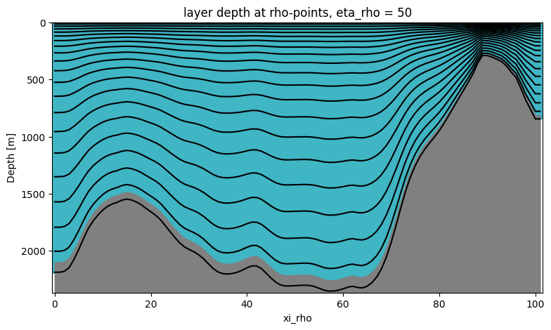
[55]:
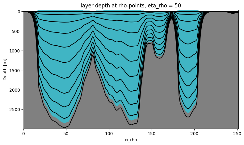
grid.plot_vertical_coordinate(eta=50)
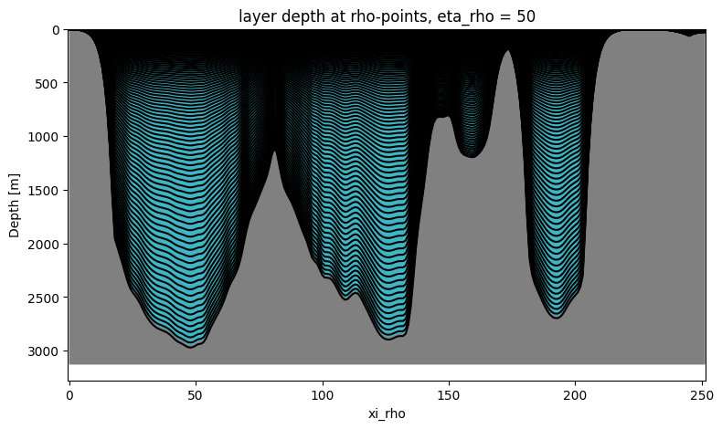
The upper ocean layers are so densely packed that the lines converge and become indistinguishable.
To address this, we offer an option to limit the number of plotted layers by specifying a maximum.
[56]:
grid.plot_vertical_coordinate(eta=50, max_nr_layer_contours=20)

Vertical coordinate system parameters#
To examine the vertical coordinate system parameters, we begin with a control grid containing just 20 vertical layers—small enough to clearly distinguish variations in the vertical plots.
[57]:
fixed_grid_parameters = {
    "nx": 100,
    "ny": 100,
    "size_x": 1800,
    "size_y": 2400,
    "center_lon": -21,
    "center_lat": 61,
    "rot": 20,
    "N": 20,
}
[58]:
control_grid = Grid(
    **fixed_grid_parameters,
    theta_s=5.0,
    theta_b=2.0,
    hc=300.0,
)
[59]:
control_grid
[59]:
Grid(nx=100, ny=100, size_x=1800, size_y=2400, center_lon=-21, center_lat=61, rot=20, N=20, theta_s=5.0, theta_b=2.0, hc=300.0, topography_source={'name': 'ETOPO5'}, close_narrow_channels=False, hmin=5.0, verbose=False, straddle=False)
We will now change the vertical coordinate system parameters theta_s, theta_b, and hc, and see what effect this has.
Critical depth#
The critical depth hc sets the transition between flat \(z\)-levels in the upper ocean and terrain-following sigma-levels below. Usually we want to choose hc to be comparable with the expected depth of the pycnocline. That being said, let’s experiment with the hc parameter.
[60]:
grid_with_large_critical_depth = Grid(
    **fixed_grid_parameters,
    theta_s=control_grid.theta_s,
    theta_b=control_grid.theta_b,
    hc=1000.0,
)

grid_with_small_critical_depth = Grid(
    **fixed_grid_parameters,
    theta_s=control_grid.theta_s,
    theta_b=control_grid.theta_b,
    hc=50.0,
)
[61]:
control_grid.plot_vertical_coordinate(eta=50)

[62]:
grid_with_large_critical_depth.plot_vertical_coordinate(eta=50)

[63]:
grid_with_small_critical_depth.plot_vertical_coordinate(eta=50)

When comparing the three plots above, we observe that
increasing
hcresults in a higher proportion of the upper ocean having nearly evenly spaced levels. It’s important to note that despite settinghcto 1000m in the second plot, the evenly spaced levels do not extend all the way down to 1000m. However, in deeper ocean regions (visible in the left part of the plot), we approach this depth threshold more closely.reducing
hcleads to a smaller proportion of the upper ocean having nearly evenly spaced levels.
Surface and bottom control parameters#
The surface control parameter theta_s and bottom control parameter theta_b determine how much the vertical grid is stretched near the surface and bottom, respectively. Let’s change these two parameters and see what happens.
[64]:
grid_with_large_theta_s = Grid(
    **fixed_grid_parameters,
    theta_s=10.0,
    theta_b=control_grid.theta_b,
    hc=control_grid.hc
)

grid_with_small_theta_s = Grid(
    **fixed_grid_parameters,
    theta_s=2.0,
    theta_b=control_grid.theta_b,
    hc=control_grid.hc
)
[65]:
control_grid.plot_vertical_coordinate(eta=50)

[66]:
grid_with_large_theta_s.plot_vertical_coordinate(eta=50)

[67]:
grid_with_small_theta_s.plot_vertical_coordinate(eta=50)

When comparing the three plots above, we can see that
increasing
theta_sleads to a refinement of the vertical grid near the surface,reducing
theta_sleads to coarsening of the vertical grid near the surface.
We can play a similar game with the bottom control parameter theta_b.
[68]:
grid_with_large_theta_b = Grid(
    **fixed_grid_parameters,
    theta_s=control_grid.theta_s,
    theta_b=6.0,
    hc=control_grid.hc
)

grid_with_small_theta_b = Grid(
    **fixed_grid_parameters,
    theta_s=control_grid.theta_s,
    theta_b=0.5,
    hc=control_grid.hc
)
[69]:
control_grid.plot_vertical_coordinate(eta=50)
[70]:
grid_with_large_theta_b.plot_vertical_coordinate(eta=50)

[71]:
grid_with_small_theta_b.plot_vertical_coordinate(eta=50)

Again, comparing the three plots above, we can see that
increasing
theta_bleads to a refinement of the vertical grid near the bottom,reducing
theta_bleads to coarsening of the vertical grid near the bottom.
Updating the vertical coordinate system#
If you want to update the vertical coordinate system but would like to keep the same horizontal grid, mask and topography, you can skip Steps I, II, and III. This can be easily achieved using the .update_vertical_coordinate method. Let’s update the grid that we created at the very beginning of this notebook.
[72]:
grid
[72]:
Grid(nx=250, ny=250, size_x=2500, size_y=2500, center_lon=-15, center_lat=65, rot=-30, N=100, theta_s=5.0, theta_b=2.0, hc=300.0, topography_source={'name': 'SRTM15', 'path': '/anvil/projects/x-ees250129/Datasets/SRTM15/SRTM15_V2.6.nc'}, close_narrow_channels=False, hmin=5.0, verbose=True, straddle=True)
[73]:
grid.update_vertical_coordinate(N=10, theta_s=1.0, verbose=True)
2026-02-08 12:09:51 - INFO - === Preparing the vertical coordinate system using N = 10, theta_s = 1.0, theta_b = 2.0, hc = 300.0 ===
2026-02-08 12:09:51 - INFO - Total time: 0.004 seconds
2026-02-08 12:09:51 - INFO - ================================================================================================
In the cell above, we regenerated the vertical coordinate system of our original grid, but this time only with 10 layers and theta_s = 1.0.
[74]:
grid
[74]:
Grid(nx=250, ny=250, size_x=2500, size_y=2500, center_lon=-15, center_lat=65, rot=-30, N=10, theta_s=1.0, theta_b=2.0, hc=300.0, topography_source={'name': 'SRTM15', 'path': '/anvil/projects/x-ees250129/Datasets/SRTM15/SRTM15_V2.6.nc'}, close_narrow_channels=False, hmin=5.0, verbose=True, straddle=True)
[75]:
grid.plot_vertical_coordinate(eta=50)