End-to-end workflow#
Tip
Prefer working in a plain Python script instead of a notebook? Download this tutorial as a .py script.
Prefer the notebook itself? Click the download button at the top of this page and choose .ipynb (not .pdf).
This notebook demonstrates an end-to-end workflow using ROMS-Tools to prepare inputs and analyze outputs for a ROMS-MARBL simulation.
We will create the following components:
Grid
Initial conditions
Surface forcing
Boundary forcing
River forcing
CDR (Carbon Dioxide Removal) forcing
After generating these inputs, we will run a ROMS-MARBL simulation and perform a basic analysis of the model output using ROMS-Tools.
Note
This notebook is intended to provide a high-level overview. For detailed explanations, see the example notebooks that explore each step individually.
Running the notebook#
To run this notebook, make sure you have the required dependencies installed. You can set them up in one of the following ways (see also this installation page):
Install with conda (recommended) — the conda-forge package includes everything this notebook needs (
xesmf, cloud-streaming and movie dependencies, and Jupyter support):conda install -c conda-forge roms-tools
Install from PyPI (e.g. on Windows, where
xesmfis not available):pip install roms-tools[stream,movie,notebooks]
Without
xesmf, regridding falls back to scipy-based methods and some features are unavailable.Install from GitHub (development):
cd roms-tools
conda env create -f ci/environment.yml
conda activate roms-tools-env
pip install -e ".[dev,stream,movie,notebooks]"
In addition, podman must be installed to run ROMS in a container. It is not a Python package and is not included in any of the installs above; see the installation instructions here.
Creating the input files with ROMS-Tools#
Let’s prepare our input data for January 2012.
[1]:
from datetime import datetime
start_time = datetime(2012, 1, 1)
end_time = datetime(2012, 1, 31)
We will save the input datasets to a designated target directory. Feel free to modify the target path!
[2]:
from pathlib import Path
[3]:
target_dir = Path("./ROMS_TOOLS_INPUT_DATA")
[4]:
# Create the directory if it doesn't exist
target_dir.mkdir(exist_ok=True)
Grid#
[5]:
from roms_tools import Grid
OMP: Info #276: omp_set_nested routine deprecated, please use omp_set_max_active_levels instead.
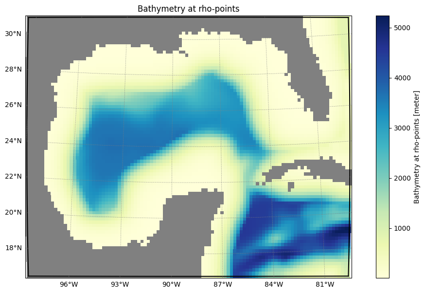
Let’s make a new domain in the Gulf of Mexico, with horizontal resolution of 20km and 20 vertical layers.
[6]:
%%time

grid = Grid(
    nx=100,  # number of grid points in x-direction
    ny=80,  # number of grid points in y-direction
    size_x=2000,  # domain size in x-direction (in km)
    size_y=1600,  # domain size in y-direction (in km)
    center_lon=-89,  # longitude of the center of the domain
    center_lat=24,  # latitude of the center of the domain
    rot=0,  # rotation of the grid (in degrees)
    N=20,  # number of vertical layers
)
CPU times: user 959 ms, sys: 62.2 ms, total: 1.02 s
Wall time: 1.12 s
Note
This example uses the default ETOPO5 bathymetry, with a horizontal resolution of 1/12°. This is sufficient for our 20 km grid, but for higher-resolution grids, consider using SRTM15. For more details on topography source data, see this page.
Let’s examine the grid variables that were created, which can be found in the xarray.Dataset returned by the .ds attribute.
[7]:
grid.ds
[7]:
<xarray.Dataset> Size: 894kB
Dimensions:       (eta_rho: 82, xi_rho: 102, xi_u: 101, eta_v: 81,
                   eta_coarse: 42, xi_coarse: 52, s_rho: 20, s_w: 21)
Coordinates:
    lat_rho       (eta_rho, xi_rho) float64 67kB 16.43 16.44 ... 30.94 30.93
    lon_rho       (eta_rho, xi_rho) float64 67kB 261.6 261.8 ... 281.3 281.5
    lat_u         (eta_rho, xi_u) float64 66kB 16.44 16.45 16.46 ... 30.95 30.93
    lon_u         (eta_rho, xi_u) float64 66kB 261.7 261.9 262.1 ... 281.2 281.4
    lat_v         (eta_v, xi_rho) float64 66kB 16.52 16.53 16.55 ... 30.85 30.84
    lon_v         (eta_v, xi_rho) float64 66kB 261.6 261.8 262.0 ... 281.3 281.5
    lat_coarse    (eta_coarse, xi_coarse) float64 17kB 16.34 16.36 ... 31.01
    lon_coarse    (eta_coarse, xi_coarse) float64 17kB 261.5 261.9 ... 281.6
Dimensions without coordinates: eta_rho, xi_rho, xi_u, eta_v, eta_coarse,
                                xi_coarse, s_rho, s_w
Data variables: (12/15)
    angle         (eta_rho, xi_rho) float64 67kB 0.06568 0.06568 ... -0.07345
    f             (eta_rho, xi_rho) float64 67kB 4.115e-05 ... 7.475e-05
    pm            (eta_rho, xi_rho) float64 67kB 5.038e-05 ... 5.038e-05
    pn            (eta_rho, xi_rho) float64 67kB 5.04e-05 5.04e-05 ... 5.04e-05
    spherical     |S1 1B b'T'
    mask_rho      (eta_rho, xi_rho) int32 33kB 0 0 0 0 0 0 0 0 ... 1 1 1 1 1 1 1
    ...            ...
    mask_coarse   (eta_coarse, xi_coarse) int32 9kB 0 0 0 0 0 0 ... 1 1 1 1 1 1
    h             (eta_rho, xi_rho) float64 67kB 5.0 5.0 5.0 ... 807.4 807.4
    sigma_r       (s_rho) float32 80B -0.975 -0.925 -0.875 ... -0.075 -0.025
    Cs_r          (s_rho) float32 80B -0.9579 -0.8615 ... -0.002245 -0.0002471
    sigma_w       (s_w) float32 84B -1.0 -0.95 -0.9 -0.85 ... -0.1 -0.05 0.0
    Cs_w          (s_w) float32 84B -1.0 -0.9114 -0.809 ... -0.0009921 0.0
Attributes: (12/14)
    title:                   ROMS grid created by ROMS-Tools
    roms_tools_version:      10000.dev364+g785fa77b7.d20260612
    size_x:                  2000
    size_y:                  1600
    center_lon:              -89
    center_lat:              24
    ...                      ...
    close_narrow_channels:   False
    topography_source_name:  ETOPO5
    hmin:                    5.0
    theta_s:                 5.0
    theta_b:                 2.0
hc: 300.0To visualize the grid we have just created, we can use the .plot method.
[8]:
grid.plot()
We can save our grid variables as a netCDF file via the .save method.
[9]:
%%time

grid.save(target_dir / "roms_grd.nc")
2026-06-23 09:14:09 - INFO - Writing the following NetCDF files:
ROMS_TOOLS_INPUT_DATA/roms_grd.nc
CPU times: user 79.1 ms, sys: 28.7 ms, total: 108 ms
Wall time: 252 ms
[9]:
[PosixPath('ROMS_TOOLS_INPUT_DATA/roms_grd.nc')]
We can also export the grid parameters to a YAML file. This gives us a more storage-effective way to save and share input data made with ROMS-Tools. The YAML file can be used to recreate the same object later.
[10]:
yaml_filepath = target_dir / "roms_grd.yaml"
grid.to_yaml(yaml_filepath)
These are the contents of the written YAML file.
[11]:
with open(yaml_filepath, "r") as file:
    file_contents = file.read()

# Print the contents
print(file_contents)
---
roms_tools_version: 10000.dev364+g785fa77b7.d20260612
---
Grid:
  nx: 100
  ny: 80
  size_x: 2000
  size_y: 1600
  center_lon: -89
  center_lat: 24
  rot: 0
  N: 20
  theta_s: 5.0
  theta_b: 2.0
  hc: 300.0
  topography_source:
    name: ETOPO5
  mask_shapefile: null
  close_narrow_channels: false
  hmin: 5.0
  parent_info: null
You can find more information about creating, plotting, and saving grids here.
Initial Conditions#
We want to prepare a simulation in which we run ROMS with MARBL biogeochemistry (BGC), so we need to prepare both physical and BGC initial conditions. We create physical and BGC initial conditions together because ROMS needs a single initial conditions file. We use
GLORYS data to create our physical initial conditions, i.e., initial temperature, salinity, sea surface height, and velocities;
a unified biogeochemical (BGC) climatology combining multiple observationally and model based sources to create our BGC initial conditions.
Here you can find instruction on how to download these datasets. We have already completed these steps, and the datasets are locally available at the paths shown below.
[12]:
glorys_path = "source-data/GoM_GLORYS_Jan2012.nc"
[13]:
unified_bgc_path = "source-data/BGCdataset_v2_1.nc"
With the source data in place, we can now generate the initial conditions.
[14]:
from roms_tools import InitialConditions
[15]:
%%time

initial_conditions = InitialConditions(
    grid=grid,
    ini_time=start_time,
    source={"name": "GLORYS", "path": glorys_path},
    bgc_source={
        "name": "UNIFIED",
        "path": unified_bgc_path,
        "climatology": True,
    },
    use_dask=True
)
2026-06-23 09:14:10 - WARNING - Optional variables missing (but not critical): ['Lig', 'DIC_ALT_CO2', 'Alk_ALT_CO2', 'temp_WOA', 'salt_WOA']
2026-06-23 09:14:10 - INFO - Density-space interpolation requested but the BGC source has no temperature/salinity; falling back to depth-space interpolation.
CPU times: user 738 ms, sys: 144 ms, total: 882 ms
Wall time: 893 ms
Note
In the cell above, we created our initial conditions with use_dask = True. This enables Dask, a Python library designated to facilitate scalable, out-of-memory data processing by distributing computations across multiple threads or processes. Here you can learn more about using Dask with ROMS-Tools.
The following variables were generated as part of the initial conditions.
[16]:
initial_conditions.ds
[16]:
<xarray.Dataset> Size: 25MB
Dimensions:      (ocean_time: 1, s_rho: 20, eta_rho: 82, xi_rho: 102,
                  xi_u: 101, eta_v: 81, s_w: 21)
Coordinates:
    abs_time     (ocean_time) datetime64[ns] 8B 2012-01-01
  * ocean_time   (ocean_time) float64 8B 3.787e+08
Dimensions without coordinates: s_rho, eta_rho, xi_rho, xi_u, eta_v, s_w
Data variables: (12/42)
    temp         (ocean_time, s_rho, eta_rho, xi_rho) float32 669kB dask.array<chunksize=(1, 20, 82, 102), meta=np.ndarray>
    salt         (ocean_time, s_rho, eta_rho, xi_rho) float32 669kB dask.array<chunksize=(1, 20, 82, 102), meta=np.ndarray>
    u            (ocean_time, s_rho, eta_rho, xi_u) float32 663kB dask.array<chunksize=(1, 20, 82, 101), meta=np.ndarray>
    v            (ocean_time, s_rho, eta_v, xi_rho) float32 661kB dask.array<chunksize=(1, 20, 81, 102), meta=np.ndarray>
    zeta         (ocean_time, eta_rho, xi_rho) float32 33kB 0.2544 ... 0.2846
    ubar         (ocean_time, eta_rho, xi_u) float32 33kB dask.array<chunksize=(1, 82, 101), meta=np.ndarray>
    ...           ...
    Lig          (ocean_time, s_rho, eta_rho, xi_rho) float32 669kB dask.array<chunksize=(1, 20, 82, 102), meta=np.ndarray>
    DIC_ALT_CO2  (ocean_time, s_rho, eta_rho, xi_rho) float32 669kB dask.array<chunksize=(1, 20, 82, 102), meta=np.ndarray>
    ALK_ALT_CO2  (ocean_time, s_rho, eta_rho, xi_rho) float32 669kB dask.array<chunksize=(1, 20, 82, 102), meta=np.ndarray>
    w            (ocean_time, s_w, eta_rho, xi_rho) float32 703kB 0.0 ... 0.0
    Cs_r         (s_rho) float32 80B -0.9579 -0.8615 ... -0.002245 -0.0002471
    Cs_w         (s_w) float32 84B -1.0 -0.9114 -0.809 ... -0.0009921 0.0
Attributes:
    title:                                ROMS initial conditions file create...
    roms_tools_version:                   10000.dev364+g785fa77b7.d20260612
    ini_time:                             2012-01-01 00:00:00
    model_reference_date:                 2000-01-01 00:00:00
    adjust_depth_for_sea_surface_height:  False
    source:                               GLORYS
    bgc_source:                           UNIFIED
    theta_s:                              5.0
    theta_b:                              2.0
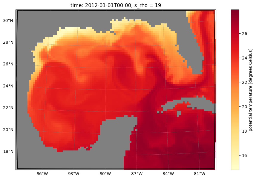
hc: 300.0Here is a plot of the uppermost layer of the temperature field.
[17]:
initial_conditions.plot("temp", s=-1)
[ ] | 0% Completed | 72.21 us[########################################] | 100% Completed | 419.43 ms
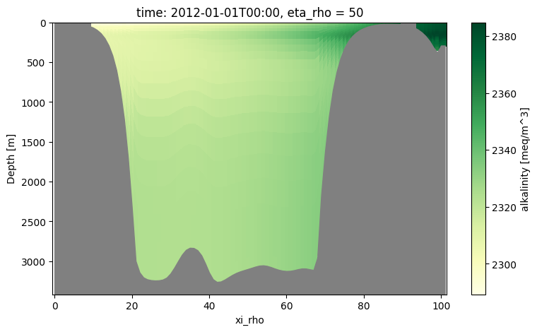
We can also plot vertical sections of our initial conditions, for example alkalinity.
[18]:
initial_conditions.plot("ALK", eta=50)
We can now save the dataset as a NetCDF and YAML file.
[19]:
initial_conditions.save(target_dir / "roms_ini.nc")
2026-06-23 09:14:11 - INFO - Writing the following NetCDF files:
ROMS_TOOLS_INPUT_DATA/roms_ini.nc
[########################################] | 100% Completed | 2.26 sms
[19]:
[PosixPath('ROMS_TOOLS_INPUT_DATA/roms_ini.nc')]
[20]:
initial_conditions.to_yaml(target_dir / "roms_ini.yaml")
You can find more information about creating, plotting, and saving initial conditions here.
Surface Forcing#
Next, we create the surface forcing for our domain.
ROMS-Tools can create two types of surface forcing:
physical surface forcing, e.g., 10m wind, shortwave radiation, and air temperature at 2m;
biogeochemical (BGC) surface forcing, e.g., atmospheric pCO2.
Unlike initial conditions data, ROMS can read multiple surface forcing files, so we create these two types separately.
[21]:
from roms_tools import SurfaceForcing
Physical Surface Forcing#
In this subsection, we use ERA5 data to generate the physical surface forcing. With ROMS-Tools, ERA5 can be streamed directly from the cloud, so you don’t need to pre-download the source data or provide a local path (though you can still do so if you prefer). See here for more details on source data options.
[22]:
%%time

surface_forcing = SurfaceForcing(
    grid=grid,
    start_time=start_time,
    end_time=end_time,
    source={"name": "ERA5"},
    type="physics",
    use_dask=True
)
2026-06-23 09:14:14 - INFO - No path specified for ERA5 source; defaulting to ARCO ERA5 dataset on Google Cloud.
2026-06-23 09:14:15 - INFO - gcsfs experimental features enabled via GCSFS_EXPERIMENTAL_ZB_HNS_SUPPORT.
2026-06-23 09:15:09 - INFO - Data will be interpolated onto the fine grid. Remember to set `interp_frc = 0` in your `bulk_frc.opt` ROMS option file.
CPU times: user 47 s, sys: 7.28 s, total: 54.2 s
Wall time: 1min 2s
Note
For an explanation of the info message about interpolation onto the fine versus coarse grid, see this page.
These are the physical surface forcing variables that were created.
[23]:
surface_forcing.ds
[23]:
<xarray.Dataset> Size: 170MB
Dimensions:   (time: 724, eta_rho: 82, xi_rho: 102)
Coordinates:
    abs_time  (time) datetime64[ns] 6kB 2011-12-31T23:00:00 ... 2012-01-31T02...
  * time      (time) float64 6kB 4.383e+03 4.383e+03 ... 4.413e+03 4.413e+03
    rad_time  (time) float64 6kB 4.383e+03 4.383e+03 ... 4.413e+03 4.413e+03
Dimensions without coordinates: eta_rho, xi_rho
Data variables:
    uwnd      (time, eta_rho, xi_rho) float32 24MB dask.array<chunksize=(1, 82, 102), meta=np.ndarray>
    vwnd      (time, eta_rho, xi_rho) float32 24MB dask.array<chunksize=(1, 82, 102), meta=np.ndarray>
    swrad     (time, eta_rho, xi_rho) float32 24MB dask.array<chunksize=(1, 82, 102), meta=np.ndarray>
    lwrad     (time, eta_rho, xi_rho) float32 24MB dask.array<chunksize=(1, 82, 102), meta=np.ndarray>
    Tair      (time, eta_rho, xi_rho) float32 24MB dask.array<chunksize=(1, 82, 102), meta=np.ndarray>
    rain      (time, eta_rho, xi_rho) float32 24MB dask.array<chunksize=(1, 82, 102), meta=np.ndarray>
    qair      (time, eta_rho, xi_rho) float32 24MB dask.array<chunksize=(1, 82, 102), meta=np.ndarray>
Attributes:
    title:                 ROMS surface forcing file created by ROMS-Tools
    roms_tools_version:    10000.dev364+g785fa77b7.d20260612
    start_time:            2012-01-01 00:00:00
    end_time:              2012-01-31 00:00:00
    source:                ERA5
    correct_radiation:     True
    wind_dropoff:          False
    use_coarse_grid:       False
    model_reference_date:  2000-01-01 00:00:00
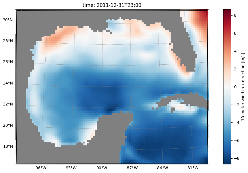
type: physicsHere is a plot of the zonal wind at the first created time stamp.
[24]:
surface_forcing.plot("uwnd", time=0)
[########################################] | 100% Completed | 519.24 ms
Let’s save our physical surface forcing to NetCDF and YAML files.
[25]:
surface_forcing.save(target_dir / "roms_frc.nc")
2026-06-23 09:15:18 - INFO - Writing the following NetCDF files:
ROMS_TOOLS_INPUT_DATA/roms_frc_201112.nc
ROMS_TOOLS_INPUT_DATA/roms_frc_201201.nc
[########################################] | 100% Completed | 842.10 ms
[########################################] | 100% Completed | 307.73 s
[25]:
[PosixPath('ROMS_TOOLS_INPUT_DATA/roms_frc_201112.nc'),
 PosixPath('ROMS_TOOLS_INPUT_DATA/roms_frc_201201.nc')]
[26]:
surface_forcing.to_yaml(target_dir / "roms_frc.yaml")
Biogeochemical (BGC) Surface Forcing#
We now create BGC surface forcing.
[27]:
%%time

bgc_surface_forcing = SurfaceForcing(
    grid=grid,
    start_time=start_time,
    end_time=end_time,
    source={"name": "UNIFIED", "path": unified_bgc_path, "climatology": True},
    type="bgc",
    use_dask=True
)
2026-06-23 09:20:35 - INFO - Data will be interpolated onto the grid coarsened by factor 2. Remember to set `interp_frc = 1` in your `bgc.opt` ROMS option file.
CPU times: user 47.1 ms, sys: 17 ms, total: 64.1 ms
Wall time: 73.5 ms
Here are the BGC surface variables that were created.
[28]:
bgc_surface_forcing.ds
[28]:
<xarray.Dataset> Size: 420kB
Dimensions:    (time: 12, eta_rho: 42, xi_rho: 52)
Coordinates:
    month      (time) int64 96B 1 2 3 4 5 6 7 8 9 10 11 12
    abs_time   (time) datetime64[ns] 96B 2000-01-16T12:00:00 ... 2000-12-15T1...
    iron_time  (time) float64 96B 15.5 45.0 74.5 105.0 ... 288.5 319.0 349.5
    dust_time  (time) float64 96B 15.5 45.0 74.5 105.0 ... 288.5 319.0 349.5
    nox_time   (time) float64 96B 15.5 45.0 74.5 105.0 ... 288.5 319.0 349.5
    nhy_time   (time) float64 96B 15.5 45.0 74.5 105.0 ... 288.5 319.0 349.5
Dimensions without coordinates: time, eta_rho, xi_rho
Data variables:
    dust       (time, eta_rho, xi_rho) float32 105kB dask.array<chunksize=(1, 42, 52), meta=np.ndarray>
    iron       (time, eta_rho, xi_rho) float32 105kB dask.array<chunksize=(1, 42, 52), meta=np.ndarray>
    nox        (time, eta_rho, xi_rho) float32 105kB dask.array<chunksize=(1, 42, 52), meta=np.ndarray>
    nhy        (time, eta_rho, xi_rho) float32 105kB dask.array<chunksize=(1, 42, 52), meta=np.ndarray>
Attributes:
    title:                 ROMS surface forcing file created by ROMS-Tools
    roms_tools_version:    10000.dev364+g785fa77b7.d20260612
    start_time:            2012-01-01 00:00:00
    end_time:              2012-01-31 00:00:00
    source:                UNIFIED
    correct_radiation:     True
    wind_dropoff:          False
    use_coarse_grid:       True
    model_reference_date:  2000-01-01 00:00:00
    type:                  bgc
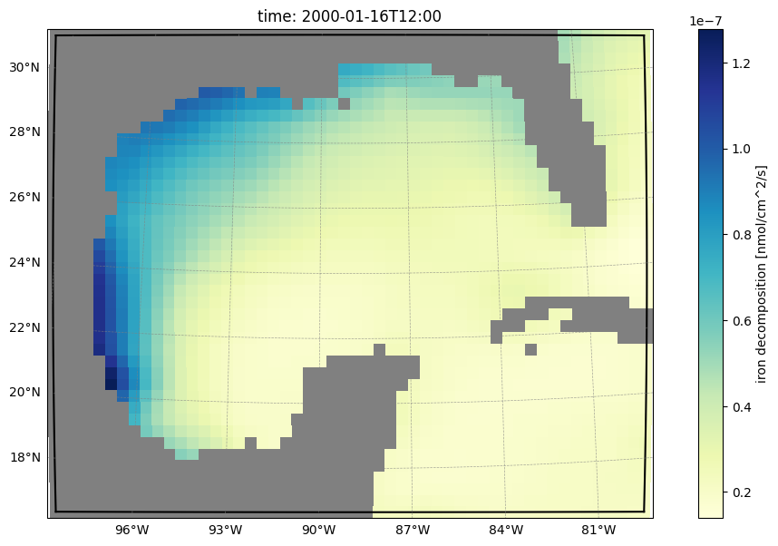
climatology: TrueLet’s plot iron, which is one of the BGC surface forcings.
[29]:
bgc_surface_forcing.plot("iron", time=0)
[########################################] | 100% Completed | 111.06 ms
Time-varying CO2#
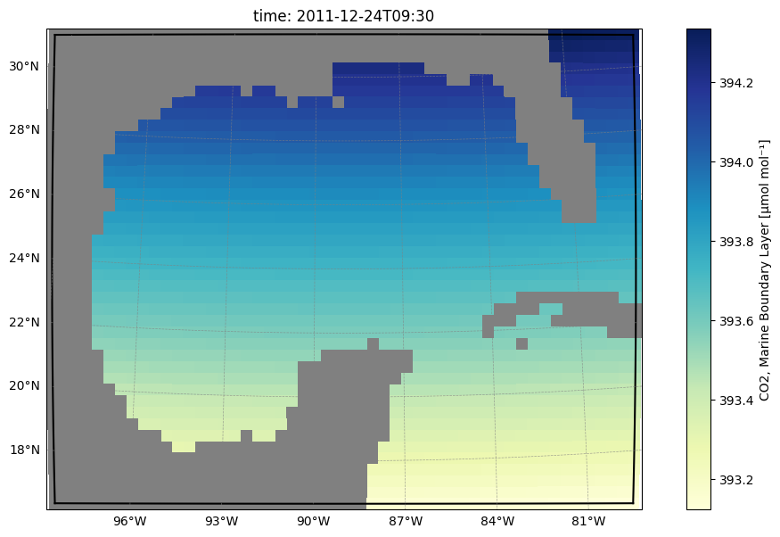
By default, ROMS assumes a constant value for the molar mixing ratio for CO2, xco2. If we would like a time-varying xco2 applied in the model, we can create a BGC surface forcing object containing xco2, similar to the BGC surface forcing generated above.
The xco2 data is interpolated from the GML’s (NOAA) Marine Boundary Layer dataset (1979-2025). For more information, see details on surface forcing. Here we let the code assume defaults.
[30]:
%%time

mbl_bgc_surface_forcing = SurfaceForcing(
    grid=grid,
    start_time=start_time,
    end_time=end_time,
    source={"name": "MBL_co2"},
    type="bgc",
)
2026-06-23 09:20:36 - INFO - No path specified for MBL_co2 source; defaulting to the MBL dataset from GML, NOAA.
2026-06-23 09:20:36 - INFO - Data will be interpolated onto the grid coarsened by factor 2. Remember to set `interp_frc = 1` in your `bgc.opt` ROMS option file.
2026-06-23 09:20:36 - INFO - Time-varying CO2 values being used.Remember to define the following flags in your `cppdefs.opt` file: {'PCO2AIR_FORCING'}`.
CPU times: user 26.7 ms, sys: 13.7 ms, total: 40.4 ms
Wall time: 59.5 ms
Here we plot a time step of xco2.
[31]:
mbl_bgc_surface_forcing.plot("xco2_air", time=0)
Finally, we save our BGC surface forcing to NetCDF and YAML files.
[32]:
bgc_surface_forcing.save(target_dir /"roms_frc_bgc.nc")
2026-06-23 09:20:36 - INFO - Writing the following NetCDF files:
ROMS_TOOLS_INPUT_DATA/roms_frc_bgc_clim.nc
[########################################] | 100% Completed | 216.65 ms
[32]:
[PosixPath('ROMS_TOOLS_INPUT_DATA/roms_frc_bgc_clim.nc')]
[33]:
bgc_surface_forcing.to_yaml(target_dir / "roms_frc_bgc.yaml")
You can find more information about creating, plotting, and saving surface forcing here.
Boundary Forcing#
In this subsection, we create the boundary forcing (or, equivalently, the open boundary conditions).
ROMS-Tools can create two types of boundary forcing:
physical boundary forcing like temperature, salinity, velocities, and sea surface height;
biogeochemical (BGC) boundary forcing like alkalinity, dissolved inorganic phosphate, etc.
As with surface forcing, ROMS accepts multiple boundary forcing files, so we create these two types separately.
[34]:
from roms_tools import BoundaryForcing
Physical boundary forcing#
We use the same GLORYS data as above to create our physical boundary forcing. Since the western boundary of our Gulf of Mexico domain lies entirely on land, we can exclude the western boundary in the following.
[35]:
%%time

boundary_forcing = BoundaryForcing(
    grid=grid,
    boundaries={
        "south": True,
        "east": True,
        "north": True,
        "west": False,   # western boundary excluded
    },
    start_time=start_time,
    end_time=end_time,
    source={"name": "GLORYS", "path": glorys_path},
    type="physics",
    use_dask=True
)
2026-06-23 09:20:36 - INFO - Using boundary configuration: {'south': True, 'east': True, 'north': True, 'west': False}
2026-06-23 09:20:36 - WARNING - No records found before the start_time: 2012-01-01 00:00:00.
2026-06-23 09:20:36 - WARNING - The southern boundary is divided by land. It would be safer (but slower and more memory-intensive) to use `apply_2d_horizontal_fill = True`.
2026-06-23 09:20:37 - WARNING - The eastern boundary is divided by land. It would be safer (but slower and more memory-intensive) to use `apply_2d_horizontal_fill = True`.
CPU times: user 770 ms, sys: 143 ms, total: 913 ms
Wall time: 899 ms
Note
Boundary data is regridded near land with a NaN-aware approach (masked bilinear interpolation plus nearest-neighbor extrapolation). See this page for details.
Here are the physical boundary forcing variables that were created.
[36]:
boundary_forcing.ds
[36]:
<xarray.Dataset> Size: 3MB
Dimensions:     (bry_time: 32, s_rho: 20, xi_u: 101, xi_rho: 102, eta_rho: 82,
                 eta_v: 81)
Coordinates:
    abs_time    (bry_time) datetime64[ns] 256B 2012-01-01 ... 2012-02-01
  * bry_time    (bry_time) float64 256B 4.383e+03 4.384e+03 ... 4.414e+03
Dimensions without coordinates: s_rho, xi_u, xi_rho, eta_rho, eta_v
Data variables: (12/21)
    u_south     (bry_time, s_rho, xi_u) float32 259kB dask.array<chunksize=(1, 20, 101), meta=np.ndarray>
    v_south     (bry_time, s_rho, xi_rho) float32 261kB dask.array<chunksize=(1, 20, 102), meta=np.ndarray>
    temp_south  (bry_time, s_rho, xi_rho) float32 261kB dask.array<chunksize=(1, 20, 102), meta=np.ndarray>
    salt_south  (bry_time, s_rho, xi_rho) float32 261kB dask.array<chunksize=(1, 20, 102), meta=np.ndarray>
    zeta_south  (bry_time, xi_rho) float32 13kB dask.array<chunksize=(1, 102), meta=np.ndarray>
    ubar_south  (bry_time, xi_u) float32 13kB dask.array<chunksize=(1, 101), meta=np.ndarray>
    ...          ...
    v_north     (bry_time, s_rho, xi_rho) float32 261kB dask.array<chunksize=(1, 20, 102), meta=np.ndarray>
    temp_north  (bry_time, s_rho, xi_rho) float32 261kB dask.array<chunksize=(1, 20, 102), meta=np.ndarray>
    salt_north  (bry_time, s_rho, xi_rho) float32 261kB dask.array<chunksize=(1, 20, 102), meta=np.ndarray>
    zeta_north  (bry_time, xi_rho) float32 13kB dask.array<chunksize=(1, 102), meta=np.ndarray>
    ubar_north  (bry_time, xi_u) float32 13kB dask.array<chunksize=(1, 101), meta=np.ndarray>
    vbar_north  (bry_time, xi_rho) float32 13kB dask.array<chunksize=(1, 102), meta=np.ndarray>
Attributes:
    title:                                ROMS boundary forcing file created ...
    roms_tools_version:                   10000.dev364+g785fa77b7.d20260612
    start_time:                           2012-01-01 00:00:00
    end_time:                             2012-01-31 00:00:00
    source:                               GLORYS
    model_reference_date:                 2000-01-01 00:00:00
    apply_2d_horizontal_fill:             False
    adjust_depth_for_sea_surface_height:  False
    theta_s:                              5.0
    theta_b:                              2.0
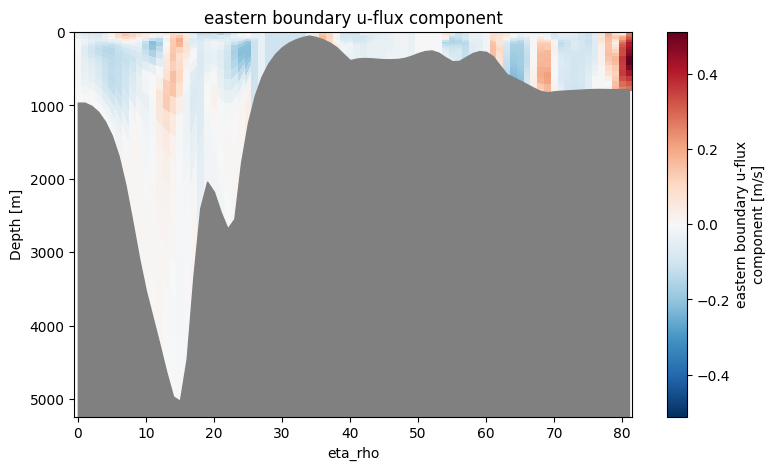
hc: 300.0Let’s plot meridional velocity at the southern boundary for the first available time stamp.
[37]:
boundary_forcing.plot("u_east", time=0)
[########################################] | 100% Completed | 111.33 ms
Finally, we save our physical boundary forcing variables to NetCDF and YAML files.
[38]:
boundary_forcing.save(target_dir / "roms_bry.nc")
2026-06-23 09:20:37 - INFO - Writing the following NetCDF files:
ROMS_TOOLS_INPUT_DATA/roms_bry_201201.nc
ROMS_TOOLS_INPUT_DATA/roms_bry_201202.nc
[########################################] | 100% Completed | 4.55 sms
[########################################] | 100% Completed | 226.27 ms
[38]:
[PosixPath('ROMS_TOOLS_INPUT_DATA/roms_bry_201201.nc'),
 PosixPath('ROMS_TOOLS_INPUT_DATA/roms_bry_201202.nc')]
[39]:
boundary_forcing.to_yaml(target_dir / "roms_bry.yaml")
Biogeochemical (BGC) boundary forcing#
We now create BGC boundary forcing. The BGC variables are interpolated from the same unified BGC climatology as above.
[40]:
%%time

bgc_boundary_forcing = BoundaryForcing(
    grid=grid,
    boundaries={
        "south": True,
        "east": True,
        "north": True,
        "west": False,   # western boundary excluded
    },
    start_time=start_time,
    end_time=end_time,
    source={"name": "UNIFIED", "path": unified_bgc_path, "climatology": True},
    type="bgc",
    use_dask=True
)
2026-06-23 09:20:42 - INFO - Using boundary configuration: {'south': True, 'east': True, 'north': True, 'west': False}
2026-06-23 09:20:42 - INFO - use_density_interpolation=True but no physics_forcing provided. BGC tracers will be interpolated in depth space instead.
2026-06-23 09:20:43 - WARNING - Optional variables missing (but not critical): ['Lig', 'DIC_ALT_CO2', 'Alk_ALT_CO2', 'temp_WOA', 'salt_WOA']
2026-06-23 09:20:43 - INFO - Density-space interpolation requested but no physics_forcing provided; falling back to depth-space interpolation (south boundary).
2026-06-23 09:20:43 - INFO - Density-space interpolation requested but no physics_forcing provided; falling back to depth-space interpolation (east boundary).
2026-06-23 09:20:43 - INFO - Density-space interpolation requested but no physics_forcing provided; falling back to depth-space interpolation (north boundary).
CPU times: user 698 ms, sys: 24.3 ms, total: 723 ms
Wall time: 767 ms
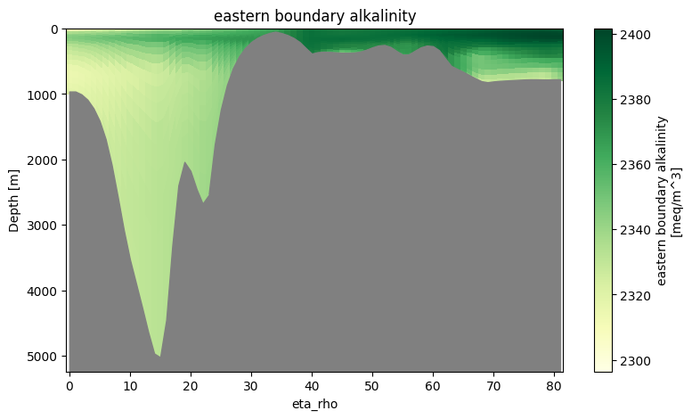
[41]:
bgc_boundary_forcing.plot("ALK_east", time=0)
[########################################] | 100% Completed | 111.05 ms
[42]:
bgc_boundary_forcing.save(target_dir / "roms_bry_bgc.nc")
2026-06-23 09:20:43 - INFO - Writing the following NetCDF files:
ROMS_TOOLS_INPUT_DATA/roms_bry_bgc_clim.nc
[########################################] | 100% Completed | 7.96 ss
[42]:
[PosixPath('ROMS_TOOLS_INPUT_DATA/roms_bry_bgc_clim.nc')]
[43]:
bgc_boundary_forcing.to_yaml(target_dir / "roms_bry_bgc.yaml")
You can find more information about creating, plotting, and saving boundary forcing here.
River Forcing#
In this subsection, we create the river forcing.
[44]:
from roms_tools import RiverForcing
[45]:
%time
river_forcing = RiverForcing(
    grid=grid,
    start_time=start_time,
    end_time=end_time,
    include_bgc=True
)
CPU times: user 1 μs, sys: 1e+03 ns, total: 2 μs
Wall time: 4.77 μs
2026-06-23 09:20:52 - INFO - No river indices provided. Identify all rivers within the ROMS domain and assign each of them to the nearest coastal point.
2026-06-23 09:20:52 - INFO - Compute climatology for river forcing.
2026-06-23 09:20:52 - WARNING - NaNs detected in 'river_volume' and set to zero. This may indicate missing river data and affect model accuracy.
Here are the river forcing variables that were created.
[46]:
river_forcing.ds
[46]:
<xarray.Dataset> Size: 134kB
Dimensions:           (ntracers: 34, river_time: 12, nriver: 34, eta_rho: 82,
                       xi_rho: 102)
Coordinates:
    tracer_name       (ntracers) <U11 1kB 'temp' 'salt' ... 'diazP' 'diazFe'
    tracer_unit       (ntracers) <U15 2kB 'degrees Celsius' 'PSU' ... 'mmol/m^3'
    tracer_long_name  (ntracers) <U43 6kB 'potential temperature' ... 'diazot...
    month             (river_time) int64 96B 1 2 3 4 5 6 7 8 9 10 11 12
    river_name        (nriver) object 272B 'Mississippi' ... 'FisheatingCree'
  * nriver            (nriver) int64 272B 1 2 3 4 5 6 7 ... 28 29 30 31 32 33 34
    abs_time          (river_time) datetime64[ns] 96B 2000-01-16 ... 2000-12-15
  * river_time        (river_time) float64 96B 15.0 45.0 74.0 ... 319.0 349.0
Dimensions without coordinates: ntracers, eta_rho, xi_rho
Data variables:
    river_volume      (river_time, nriver) float32 2kB 2.12e+04 ... 1.927
    river_tracer      (river_time, ntracers, nriver) float32 55kB 17.0 ... 1....
    river_index       (eta_rho, xi_rho) float32 33kB 0.0 0.0 0.0 ... 0.0 0.0 0.0
    river_fraction    (eta_rho, xi_rho) float32 33kB 0.0 0.0 0.0 ... 0.0 0.0 0.0
Attributes:
climatology: TrueLet’s make a plot of the river locations.
[47]:
river_forcing.plot_locations()
2026-06-23 09:20:52 - WARNING - Only the first 20 rivers will be plotted (received 34).
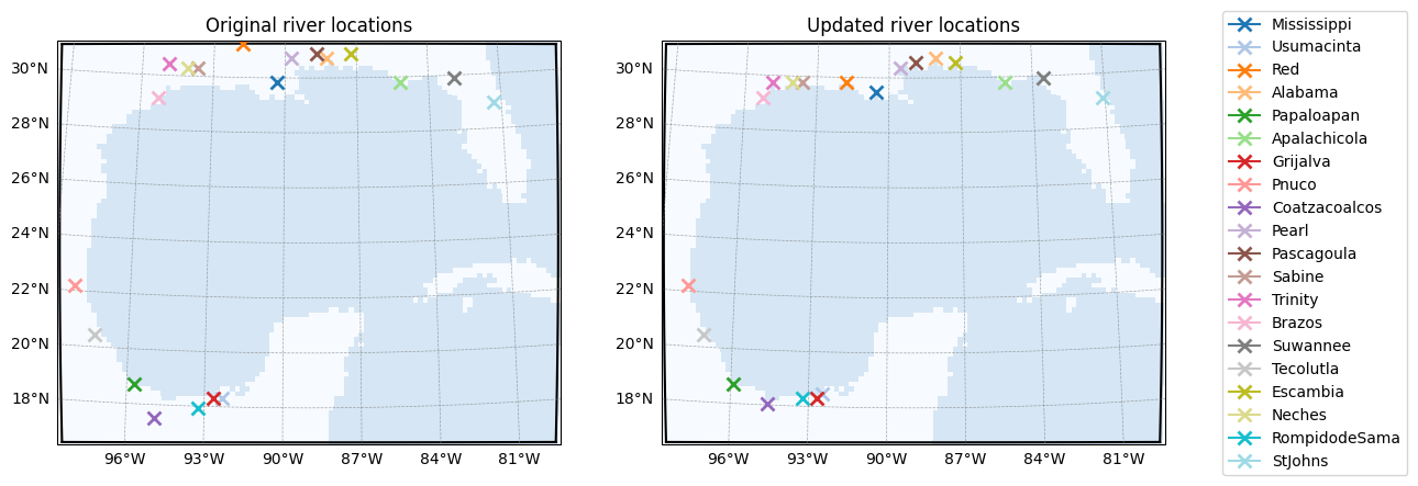
The left plot shows the original river locations from the Dai and Trenberth global river dataset mapped onto the ROMS domain, many of which are off the coast. ROMS requires rivers to be on land adjacent to wet points. The right plot shows the updated locations, where ROMS-Tools shifted each river to the nearest coastal grid point.
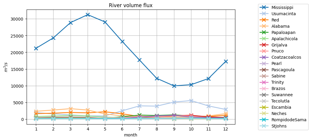
Let’s make a plot of the volume flux for the rivers shown above.
[48]:
river_forcing.plot("river_volume")
2026-06-23 09:20:53 - WARNING - Only the first 20 rivers will be plotted (received 34).
Finally, we save the river forcing to NetCDF and YAML files.
[49]:
river_forcing.save(target_dir / "roms_rivers.nc")
2026-06-23 09:20:53 - INFO - Writing the following NetCDF files:
ROMS_TOOLS_INPUT_DATA/roms_rivers.nc
[49]:
[PosixPath('ROMS_TOOLS_INPUT_DATA/roms_rivers.nc')]
[50]:
river_forcing.to_yaml(target_dir / "roms_rivers.yaml")
You can find more information about creating, plotting, and saving river forcing here.
Carbon Dioxide Removal (CDR) Forcing#
Lastly, we create CDR forcing for our simulation.
[51]:
from roms_tools import TracerPerturbation, CDRForcing
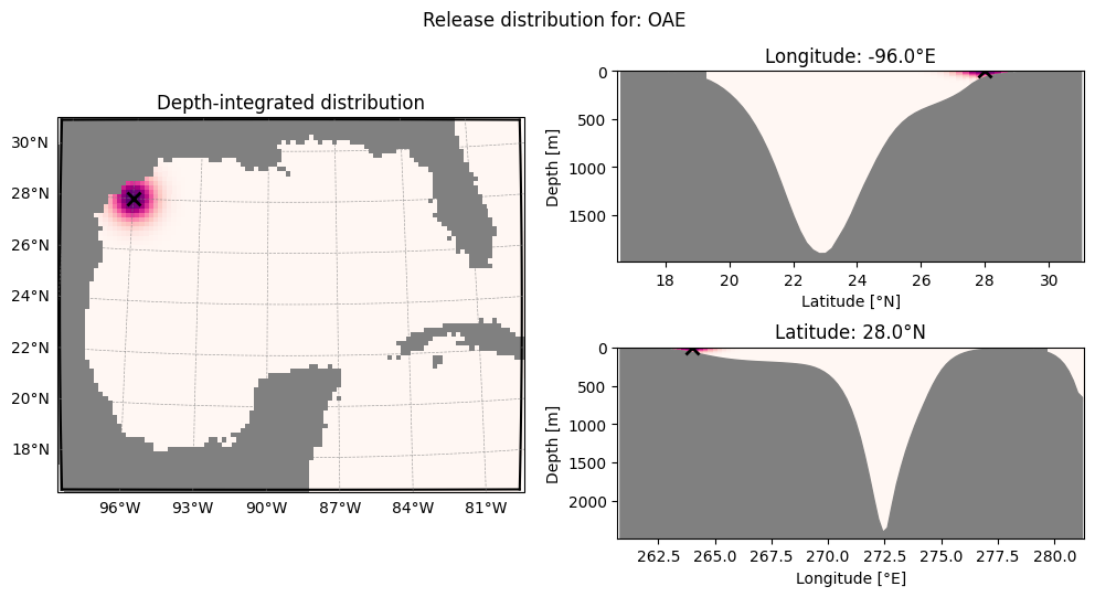
We first define a tracer perturbation release, which perturbs the BGC tracer fields without adding water. This approach is suitable for large-scale applications where mixing has already occurred, such as in a pre-run mixing model.
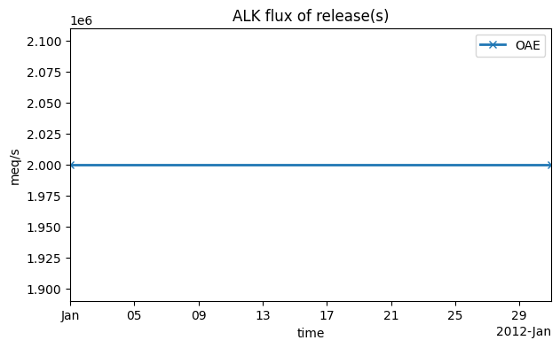
The perturbation is centered at 28°N, 96°W, and at the surface (0 m depth). It is distributed using a Gaussian with standard deviations of 100 km horizontally and 50 m vertically. We release an alkalinity flux of 2,000,000 meq/s over the entire simulation period.
[52]:
release = TracerPerturbation(
    name="OAE",
    lat=28,  # degree N
    lon=-96,  # degree E
    depth=0,  # m
    hsc=100000, # m
    vsc=50,  # m
    tracer_fluxes={"ALK": 2 * 10**6},  # meq/s
)
For more complex, time-varying releases, or releases that add water in addition to perturbing tracers (relevant for field-scale deployments where mixing is still required), see this page.
We now assemble all releases that we want to run in a single simulations into the CDR forcing.
[53]:
cdr_forcing = CDRForcing(
    grid=grid,
    start_time=start_time, # simulation start time
    end_time=end_time, # simulation end time
    releases=[release]
)
We can make a plot of the release distribution.
[54]:
cdr_forcing.plot_distribution(release_name="OAE")
Here is a plot of the alkalinity flux being released, which is constant over time.
[55]:
cdr_forcing.plot_tracer_flux(tracer_name="ALK")
Finally, we save the CDR forcing to NetCDF and YAML files.
[56]:
cdr_forcing.save(target_dir / "roms_cdr.nc")
2026-06-23 09:20:54 - INFO - Writing the following NetCDF files:
ROMS_TOOLS_INPUT_DATA/roms_cdr.nc
[56]:
[PosixPath('ROMS_TOOLS_INPUT_DATA/roms_cdr.nc')]
[57]:
cdr_forcing.to_yaml(target_dir / "roms_cdr.yaml")
Running ROMS#
In the last section we have made all necessary input fields. We are now ready to run a ROMS-MARBL simulation!
Here we run a pre-compiled version of ROMS using a container. Containers can be used to run programs in portable, reproducible pre-configured environments.
Note
This precompiled ROMS executable is built specifically for this example. As a result, compile-time options, such as the horizontal grid dimensions (nx, ny) used in this notebook, cannot be modified and still be expected to work with the precompiled ROMS executable in the container.
Let’s first make a directory that will hold the model output.
[58]:
from pathlib import Path
[59]:
output_dir = Path("./OUTPUT")
[60]:
output_dir.mkdir(exist_ok=True)
Next, users on MacOS must first initialise a virtual machine. Make sure that podman is installed, as noted at the top of the notebook.
[61]:
import os
[62]:
os.environ["PATH"] = "/opt/podman/bin:" + os.environ["PATH"]
[63]:
%%bash

podman machine init --cpus 10
podman machine start
Error: podman-machine-default: VM already exists
Starting machine "podman-machine-default"

This machine is currently configured in rootless mode. If your containers
require root permissions (e.g. ports < 1024), or if you run into compatibility
issues with non-podman clients, you can switch using the following command:

        podman machine set --rootful

API forwarding listening on: /var/folders/0f/07hq__ls2tdgjy7vykrfmmch0000gn/T/podman/podman-machine-default-api.sock

The system helper service is not installed; the default Docker API socket
address can't be used by podman. If you would like to install it, run the following commands:

        sudo /opt/homebrew/Cellar/podman/5.8.2/bin/podman-mac-helper install
        podman machine stop; podman machine start

You can still connect Docker API clients by setting DOCKER_HOST using the
following command in your terminal session:

        export DOCKER_HOST='unix:///var/folders/0f/07hq__ls2tdgjy7vykrfmmch0000gn/T/podman/podman-machine-default-api.sock'

Machine "podman-machine-default" started successfully
We have built a container for this example that is available through the GitHub Container Repository. Let’s pull this container image!
[64]:
%%bash

podman pull ghcr.io/cworthy-ocean/roms_tools_end_to_end_example:latest > /dev/null 2>&1
In the above cell, the > /dev/null 2>&1 part suppresses all output. Remove it if you want to see the download progress and logs.
Now we can run the container with the following flags:
--rm: automatically remove the container after it finishes-v: mount directories for input files and output so ROMS-MARBL can access inputs and save results
We prefix the command with time to measure how long the simulation takes to run.
[ ]:
%%bash

podman run --rm -v ./ROMS_TOOLS_INPUT_DATA:/input -v ./OUTPUT:/output ghcr.io/cworthy-ocean/roms_tools_end_to_end_example:latest > /dev/null 2>&1
Again, the > /dev/null 2>&1 part suppresses all output. Remove it if you want to see the full (and very long) ROMS model output.
Analyzing the output#
The output is now in the OUTPUT directory that we created.
[ ]:
ls OUTPUT/
ROMS_example_cstar.20120102000000.nc ROMS_example_his.20120101000000.nc
The ROMS_example_his*.nc files contain snapshots of the physical variables, while the ROMS_example_cstar*.nc files hold the CDR-related output.
We can visualize the output with ROMS-Tools.
[ ]:
from roms_tools import ROMSOutput
Let’s first look at the snapshots of the physical variables.
[ ]:
roms_output = ROMSOutput(
    grid=grid,
    path="OUTPUT/ROMS_example_his.20120101000000.nc",
    use_dask=True,
)
This output contains 31 snapshots, one per day.
[ ]:
roms_output.ds
<xarray.Dataset> Size: 86MB
Dimensions:     (time: 31, auxil: 6, eta_rho: 82, xi_rho: 102, xi_u: 101,
                 eta_v: 81, s_rho: 20)
Coordinates:
    abs_time    (time) datetime64[ns] 248B 2012-01-01 2012-01-02 ... 2012-01-31
    lat_rho     (eta_rho, xi_rho) float64 67kB 16.43 16.44 16.46 ... 30.94 30.93
    lon_rho     (eta_rho, xi_rho) float64 67kB 261.6 261.8 262.0 ... 281.3 281.5
    lat_u       (eta_rho, xi_u) float64 66kB 16.44 16.45 16.46 ... 30.95 30.93
    lon_u       (eta_rho, xi_u) float64 66kB 261.7 261.9 262.1 ... 281.2 281.4
    lat_v       (eta_v, xi_rho) float64 66kB 16.52 16.53 16.55 ... 30.85 30.84
    lon_v       (eta_v, xi_rho) float64 66kB 261.6 261.8 262.0 ... 281.3 281.5
Dimensions without coordinates: time, auxil, eta_rho, xi_rho, xi_u, eta_v, s_rho
Data variables:
    ocean_time  (time) float64 248B dask.array<chunksize=(1,), meta=np.ndarray>
    time_step   (time, auxil) int32 744B dask.array<chunksize=(1, 6), meta=np.ndarray>
    zeta        (time, eta_rho, xi_rho) float32 1MB dask.array<chunksize=(1, 82, 102), meta=np.ndarray>
    ubar        (time, eta_rho, xi_u) float32 1MB dask.array<chunksize=(1, 82, 101), meta=np.ndarray>
    vbar        (time, eta_v, xi_rho) float32 1MB dask.array<chunksize=(1, 81, 102), meta=np.ndarray>
    u           (time, s_rho, eta_rho, xi_u) float32 21MB dask.array<chunksize=(1, 20, 82, 101), meta=np.ndarray>
    v           (time, s_rho, eta_v, xi_rho) float32 20MB dask.array<chunksize=(1, 20, 81, 102), meta=np.ndarray>
    temp        (time, s_rho, eta_rho, xi_rho) float32 21MB dask.array<chunksize=(1, 20, 82, 102), meta=np.ndarray>
    salt        (time, s_rho, eta_rho, xi_rho) float32 21MB dask.array<chunksize=(1, 20, 82, 102), meta=np.ndarray>
Attributes: (12/44)
    global_x:           100
    global_y:           80
    title:              Example run
    grid_file:          ROMS_TOOLS_INPUT_DATA/roms_grd.0.nc
    forcing_files:       ROMS_TOOLS_INPUT_DATA/roms_frc_201201.0.nc ROMS_TOOL...
    forcing_info:
    ...                 ...
    tide_options:       OFF
    river_frc_options:  OFF
    pipe_frc_options:   OFF
    particle_options:   OFF
    git_version:        eeaca4861898a27443cd1f693811c321140ef58c
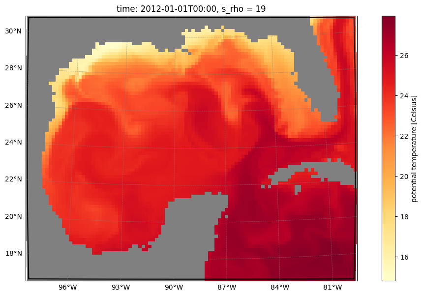
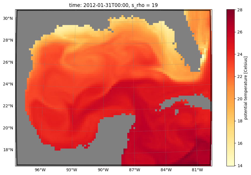
type: ROMS history fileLet’s plot the sea surface temperature at the start of the simulation (January 1, 2012) and again 31 days later.
[ ]:
roms_output.plot("temp", s=-1, time=0)
[########################################] | 100% Completed | 106.28 ms
[ ]:
roms_output.plot("temp", s=-1, time=-1)
[########################################] | 100% Completed | 103.00 ms
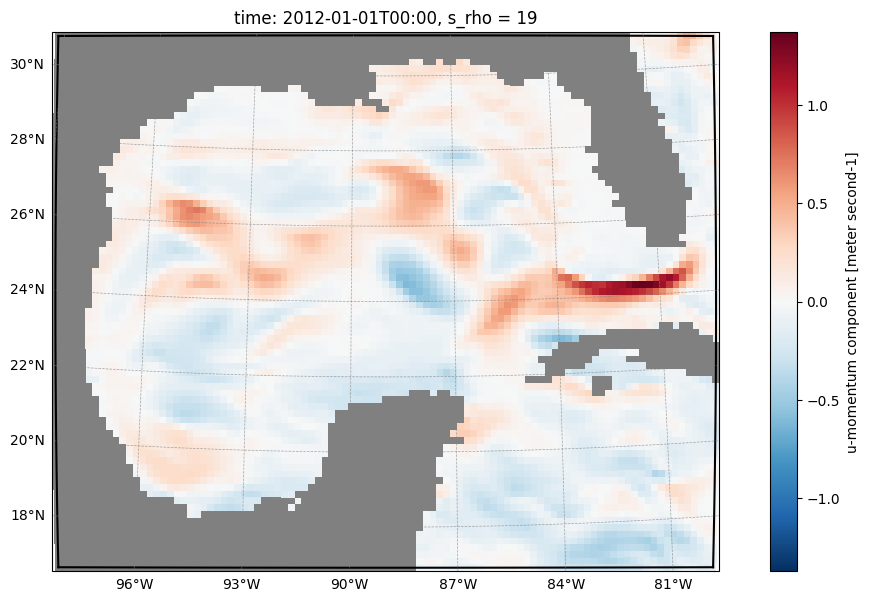
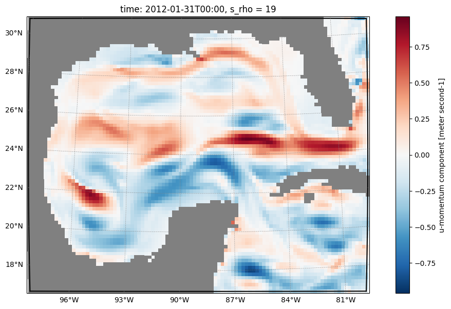
We can also compare zonal surface velocity at the start of the simulation and 31 days later.
[ ]:
roms_output.plot("u", s=-1, time=0)
[########################################] | 100% Completed | 106.18 ms
[ ]:
roms_output.plot("u", s=-1, time=-1)
[########################################] | 100% Completed | 105.55 ms
You can learn more about visualizing ROMS output here.
Let’s now have a look at the CDR-related output.
[ ]:
cdr_roms_output = ROMSOutput(
    grid=grid,
    path="OUTPUT/ROMS_example_cstar.20120102000000.nc",
    use_dask=True,
)
This output contains 30 time stamps, each representing a daily average.
[ ]:
cdr_roms_output.ds
<xarray.Dataset> Size: 649MB
Dimensions:         (time: 30, eta_rho: 82, xi_rho: 102, s_rho: 20)
Coordinates:
    abs_time        (time) datetime64[ns] 240B 2012-01-02 ... 2012-01-31
    lat_rho         (eta_rho, xi_rho) float64 67kB 16.43 16.44 ... 30.94 30.93
    lon_rho         (eta_rho, xi_rho) float64 67kB 261.6 261.8 ... 281.3 281.5
Dimensions without coordinates: time, eta_rho, xi_rho, s_rho
Data variables: (12/22)
    ocean_time      (time) float64 240B dask.array<chunksize=(1,), meta=np.ndarray>
    zeta            (time, eta_rho, xi_rho) float64 2MB dask.array<chunksize=(1, 82, 102), meta=np.ndarray>
    temp            (time, s_rho, eta_rho, xi_rho) float64 40MB dask.array<chunksize=(1, 20, 82, 102), meta=np.ndarray>
    salt            (time, s_rho, eta_rho, xi_rho) float64 40MB dask.array<chunksize=(1, 20, 82, 102), meta=np.ndarray>
    ALK             (time, s_rho, eta_rho, xi_rho) float64 40MB dask.array<chunksize=(1, 20, 82, 102), meta=np.ndarray>
    DIC             (time, s_rho, eta_rho, xi_rho) float64 40MB dask.array<chunksize=(1, 20, 82, 102), meta=np.ndarray>
    ...              ...
    ALK_source      (time, s_rho, eta_rho, xi_rho) float64 40MB dask.array<chunksize=(1, 20, 82, 102), meta=np.ndarray>
    ALK_ALT_source  (time, s_rho, eta_rho, xi_rho) float64 40MB dask.array<chunksize=(1, 20, 82, 102), meta=np.ndarray>
    DIC_source      (time, s_rho, eta_rho, xi_rho) float64 40MB dask.array<chunksize=(1, 20, 82, 102), meta=np.ndarray>
    DIC_ALT_source  (time, s_rho, eta_rho, xi_rho) float64 40MB dask.array<chunksize=(1, 20, 82, 102), meta=np.ndarray>
    avg_begin_time  (time) float64 240B dask.array<chunksize=(1,), meta=np.ndarray>
    avg_end_time    (time) float64 240B dask.array<chunksize=(1,), meta=np.ndarray>
Attributes: (12/44)
    global_x:           100
    global_y:           80
    title:              Example run
    grid_file:          ROMS_TOOLS_INPUT_DATA/roms_grd.0.nc
    forcing_files:       ROMS_TOOLS_INPUT_DATA/roms_frc_201201.0.nc ROMS_TOOL...
    forcing_info:
    ...                 ...
    tide_options:       OFF
    river_frc_options:  OFF
    pipe_frc_options:   OFF
    particle_options:   OFF
    git_version:        eeaca4861898a27443cd1f693811c321140ef58c
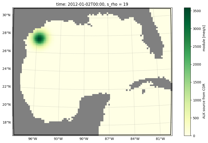
averaging: All variables are averaged in timeHere we show the alkalinity source term diagnosed online by the model, plotted at the surface for the first time step.
[ ]:
cdr_roms_output.plot("ALK_source", s=-1, time=0)
[########################################] | 100% Completed | 104.26 ms
Finally, we compute the CDR uptake curves using two approaches: from CO₂ flux differences and from DIC differences. A more detailed explanation is provided here.
[ ]:
cdr_roms_output.cdr_metrics()
2025-09-29 16:08:22 - INFO - Max absolute difference between flux-based and DIC-based uptake efficiency: 4.559e-03
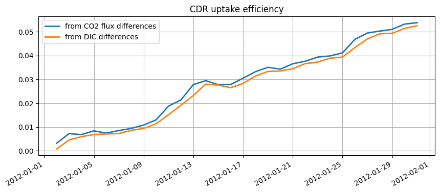
There are slight differences between the uptake curves depending on the computation method, but overall they agree closely. Since the simulation was run for only one month, the uptake efficiency remains relatively low, around 5% at the end of the period. Extending the simulation would allow the efficiency to increase further.
The computed CDR metrics can also be found in the .ds_cdr attribute.
[ ]:
cdr_roms_output.ds_cdr
<xarray.Dataset> Size: 85MB
Dimensions:                         (time: 30, eta_rho: 82, xi_rho: 102,
                                     s_rho: 20)
Coordinates:
    abs_time                        (time) datetime64[ns] 240B 2012-01-02 ......
    lat_rho                         (eta_rho, xi_rho) float64 67kB 16.43 ... ...
    lon_rho                         (eta_rho, xi_rho) float64 67kB 261.6 ... ...
Dimensions without coordinates: time, eta_rho, xi_rho, s_rho
Data variables:
    FG_CO2                          (time, eta_rho, xi_rho) float64 2MB dask.array<chunksize=(1, 82, 102), meta=np.ndarray>
    FG_ALT_CO2                      (time, eta_rho, xi_rho) float64 2MB dask.array<chunksize=(1, 82, 102), meta=np.ndarray>
    hDIC                            (time, s_rho, eta_rho, xi_rho) float64 40MB dask.array<chunksize=(1, 20, 82, 102), meta=np.ndarray>
    hDIC_ALT_CO2                    (time, s_rho, eta_rho, xi_rho) float64 40MB dask.array<chunksize=(1, 20, 82, 102), meta=np.ndarray>
    area                            (eta_rho, xi_rho) float64 67kB 3.938e+08 ...
    window_length                   (time) float64 240B dask.array<chunksize=(1,), meta=np.ndarray>
    cdr_efficiency                  (time) float64 240B dask.array<chunksize=(1,), meta=np.ndarray>
cdr_efficiency_from_delta_diff (time) float64 240B dask.array<chunksize=(1,), meta=np.ndarray>Learn more about analyzing CDR metrics here.
[ ]: