Preparing nested simulations#
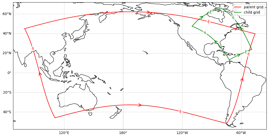
Running a nested ROMS simulation involves setting up a parent grid (red outline) and a child grid (green outline), as illustrated in the figure below.

Proper preparation of a nested simulation can significantly save computation time and ensure smooth integration between the parent and child simulations. The necessary steps are as follows:
Steps Before Running the Parent Simulation:
Adjust Child Grid Topography and Mask: The topography and mask of the child grid need to be adjusted such that they align with the parent grid at the child boundaries.
Map Child Grid Boundaries: The boundaries of the child grid must be mapped onto the parent grid’s indices and saved in a NetCDF file. This file instructs ROMS to output the parent simulation state at the child grid boundaries at a specified frequency.
Steps Before Running the Child Simulation:
Prepare Boundary Forcing: Boundary forcing for the child simulation is generated from the parent simulation’s state, which was output as a result of the preparation in Step 2.
Regrid Initial Conditions: Initial conditions for the child simulation are regridded from the parent simulation results.
This notebook guides you through these four steps.
Creating the parent child grid#
[1]:
from roms_tools import Grid, align_grids, make_nesting_info
First, we create a parent grid using the Grid class, as usual.
[2]:
parent_grid = Grid(
    nx=200,
    ny=200,
    size_x=2500,
    size_y=3000,
    center_lon=-30,
    center_lat=57,
    rot=-20,
    topography_source={
        "name": "SRTM15",
        "path": "/anvil/projects/x-ees250129/Datasets/SRTM15/SRTM15_V2.6.nc",
    },
)
[3]:
parent_grid.plot()

Next, we create a child grid, also using the Grid class.
[4]:
child_grid_parameters = {
    "nx": 500,
    "ny": 500,
    "size_x": 400,
    "size_y": 400,
    "center_lon": -25,
    "center_lat": 65.5,
    "rot": 10,
    "topography_source": {
        "name": "SRTM15",
        "path": "/anvil/projects/x-ees250129/Datasets/SRTM15/SRTM15_V2.6.nc"
    },
}
[5]:
child_grid = Grid(**child_grid_parameters)
[6]:
child_grid.plot()

As usual for Grid objects, both the parent and child grid have a .ds attribute, which contains an xarray Dataset that holds all the grid variables.
[7]:
child_grid.ds
[7]:
<xarray.Dataset> Size: 27MB
Dimensions:       (eta_rho: 502, xi_rho: 502, xi_u: 501, eta_v: 501,
                   eta_coarse: 252, xi_coarse: 252, s_rho: 100, s_w: 101)
Coordinates:
    lat_rho       (eta_rho, xi_rho) float64 2MB 63.37 63.38 ... 67.54 67.54
    lon_rho       (eta_rho, xi_rho) float64 2MB 331.7 331.8 ... 338.8 338.8
    lat_u         (eta_rho, xi_u) float64 2MB 63.38 63.38 63.38 ... 67.54 67.54
    lon_u         (eta_rho, xi_u) float64 2MB 331.7 331.8 331.8 ... 338.8 338.8
    lat_v         (eta_v, xi_rho) float64 2MB 63.38 63.38 63.38 ... 67.54 67.54
    lon_v         (eta_v, xi_rho) float64 2MB 331.7 331.8 331.8 ... 338.8 338.8
    lat_coarse    (eta_coarse, xi_coarse) float64 508kB 63.37 63.37 ... 67.55
    lon_coarse    (eta_coarse, xi_coarse) float64 508kB 331.7 331.8 ... 338.8
Dimensions without coordinates: eta_rho, xi_rho, xi_u, eta_v, eta_coarse,
                                xi_coarse, s_rho, s_w
Data variables: (12/15)
    angle         (eta_rho, xi_rho) float64 2MB 0.2261 0.2261 ... 0.114 0.114
    f             (eta_rho, xi_rho) float64 2MB 0.00013 0.00013 ... 0.0001344
    pm            (eta_rho, xi_rho) float64 2MB 0.001251 0.001251 ... 0.001251
    pn            (eta_rho, xi_rho) float64 2MB 0.001251 0.001251 ... 0.001251
    spherical     |S1 1B b'T'
    mask_rho      (eta_rho, xi_rho) int32 1MB 1 1 1 1 1 1 1 1 ... 1 1 1 1 1 1 1
    ...            ...
    mask_coarse   (eta_coarse, xi_coarse) int32 254kB 1 1 1 1 1 1 ... 1 1 1 1 1
    h             (eta_rho, xi_rho) float64 2MB 1.642e+03 1.642e+03 ... 635.1
    sigma_r       (s_rho) float32 400B -0.995 -0.985 -0.975 ... -0.015 -0.005
    Cs_r          (s_rho) float32 400B -0.992 -0.9753 ... -8.89e-05 -9.874e-06
    sigma_w       (s_w) float32 404B -1.0 -0.99 -0.98 -0.97 ... -0.02 -0.01 0.0
    Cs_w          (s_w) float32 404B -1.0 -0.9837 -0.9667 ... -3.95e-05 0.0
Attributes: (12/15)
    title:                   ROMS grid created by ROMS-Tools
    roms_tools_version:      3.6.1.dev31+g34326e51e
    size_x:                  400
    size_y:                  400
    center_lon:              -25
    center_lat:              65.5
    ...                      ...
    topography_source_name:  SRTM15
    topography_source_path:  /anvil/projects/x-ees250129/Datasets/SRTM15/SRTM...
    hmin:                    5.0
    theta_s:                 5.0
    theta_b:                 2.0
hc: 300.0Plot nested domains#
We can plot the parent and child grids together with the plot_nesting function to visualize their relative positions.
[8]:
from roms_tools import plot_nesting
plot_nesting(parent_grid, child_grid, with_dim_names=True)

Adjust Child Grid Topography and Mask#
Steps 1 and 2 from above are performed by the ROMS-Tools functions align_grids and make_nesting_info. To perform step 1, we use the align_grids function.
[9]:
child_grid = align_grids(parent_grid=parent_grid, child_grid=child_grid, verbose=True)
2026-04-16 14:13:34 - INFO - No `boundaries` provided. Using mask-based defaults: {'south': True, 'east': True, 'north': True, 'west': True}
2026-04-16 14:13:39 - INFO - === Modifying the child mask ===
2026-04-16 14:13:39 - INFO - Total time: 0.514 seconds
2026-04-16 14:13:39 - INFO - ================================================================================================
2026-04-16 14:13:39 - INFO - === Modifying the child topography ===
2026-04-16 14:13:40 - INFO - Total time: 0.514 seconds
2026-04-16 14:13:40 - INFO - ================================================================================================
Adjusted topography and mask#
Let’s examine the outcome of Step 1, where the child grid’s topography (or bathymetry) and mask have been adjusted to align with the parent grid. Above, we plotted the bathymetry of our child grid. For comparison, here is another grid with the same parameters as our child grid, but not updated to smooth into a parent grid.
[10]:
child_grid_without_parent = Grid(**child_grid_parameters)
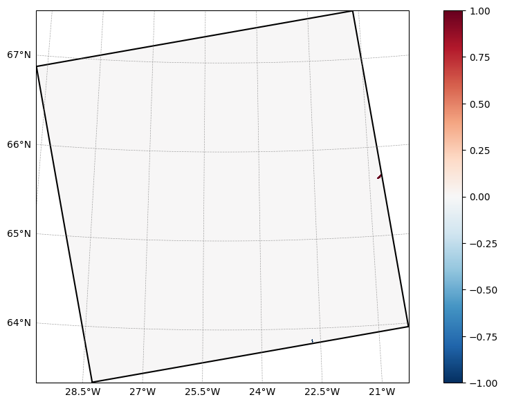
We can visualize the difference between the two bathymetries of our child grid (with and without a parent grid) by plotting their difference. The parent grid object provides the reference for the child grid’s topography and mask, and the boundaries of the child grid are adapted to smooth the transition.
[11]:
from roms_tools.plot import plot
plot(child_grid.ds["h"] - child_grid_without_parent.ds["h"], grid_ds=child_grid.ds, cmap_name="RdBu_r")

The topography modifications are concentrated near the boundaries. Everywhere else, the child topography remains unchanged.
The mask of the child grid with parent has also been adjusted along the boundaries (in comparison to the child grid without a parent) to better align with the mask of the parent grid.
[12]:
plot(child_grid.ds["mask_rho"] - child_grid_without_parent.ds["mask_rho"], grid_ds=child_grid.ds, apply_mask=False, cmap_name="RdBu_r")
Child grid boundaries mapped onto parent grid indices#
The boundaries of the child grid need to be mapped onto the parent grid’s indices (Step 2) so that the results from the parent grid can be passed to the child grid. To do so, we use the make_nesting_info function.
[13]:
prefix = 'child'
period = 3600
include_bgc = False
include_pressure_fluxes = False

filepath = '/anvil/scratch/x-smaticka/sims_runtime/nesting/nesting_info.nc'
ds_nesting = make_nesting_info(parent_grid=parent_grid, child_grid=child_grid, filepath=filepath, prefix=prefix, period=period, include_bgc=include_bgc, include_pressure_fluxes=include_pressure_fluxes, verbose=True)
2026-04-16 14:13:50 - INFO - No `boundaries` provided. Using mask-based defaults: {'south': True, 'east': True, 'north': True, 'west': True}
2026-04-16 14:13:50 - INFO - === Mapping the child grid boundary points onto the indices of the parent grid ===
2026-04-16 14:14:04 - INFO - Total time: 13.182 seconds
2026-04-16 14:14:04 - INFO - ================================================================================================
2026-04-16 14:14:04 - INFO - Writing the following NetCDF files:
/anvil/scratch/x-smaticka/sims_runtime/nesting/nesting_info.nc
The indexed boundaries are now stored in an xarray.Dataset accessible via the ds_nesting dataset, they are also saved to the filepath prescribed. If it is not desired to save a file, filepath can be set to None in make_nesting_info.
Notice that the make_nesting_info function requires a few parameters in addition to the parent and child grids:
boundaries: Specifies which of the child grid’s boundaries are open (south,east,north,west). NOTE: If omitted,ROMS-Toolswill automatically infer them based on the land/sea mask. This affects two aspects:The specified boundaries are adjusted to match the parent grid’s topography and mask.
The specified boundaries are mapped onto parent grid indices.
The following are configuration details related to boundary mapping and nesting behavior:
prefix: A string used as the prefix for child-grid variables in the boundary-mapping output. When using the Fortran toolextract_data_jointo convert the model-generated.extfiles into boundary forcing files, this same prefix is also applied to the resulting file names, for example:"prefix"_bry.20241006000240.nc.period: The temporal resolution (in seconds) for boundary outputs. Defaults to 3600 (hourly).include_bgc: Whether to include BGC variables in the boundary mapping. Defaults to False.include_pressure_fluxes: Whether to include pressure fluxes in the boundary mapping. Defaults to False.
[14]:
ds_nesting
[14]:
<xarray.Dataset> Size: 128kB
Dimensions:        (two: 2, child_xi_rho: 502, three: 3, child_xi_u: 501,
                    child_eta_rho: 502, child_eta_v: 501)
Dimensions without coordinates: two, child_xi_rho, three, child_xi_u,
                                child_eta_rho, child_eta_v
Data variables:
    child_south_r  (two, child_xi_rho) float64 8kB 87.12 87.18 ... 160.5 160.5
    child_south_u  (three, child_xi_u) float64 12kB 87.15 87.2 ... 0.09919
    child_south_v  (three, child_xi_rho) float64 12kB 87.11 87.16 ... 0.0992
    child_east_r   (two, child_eta_rho) float64 8kB 105.5 105.5 ... 183.6 183.6
    child_east_u   (three, child_eta_rho) float64 12kB 105.4 105.4 ... 0.114
    child_east_v   (three, child_eta_v) float64 12kB 105.4 105.4 ... 0.114 0.114
    child_north_r  (two, child_xi_rho) float64 8kB 69.02 69.07 ... 183.6 183.6
    child_north_u  (three, child_xi_u) float64 12kB 69.05 69.1 ... 0.1142 0.114
    child_north_v  (three, child_xi_rho) float64 12kB 69.04 69.09 ... 0.114
    child_west_r   (two, child_eta_rho) float64 8kB 87.12 87.09 ... 168.5 168.5
    child_west_u   (three, child_eta_rho) float64 12kB 87.15 87.11 ... 0.2587
child_west_v (three, child_eta_v) float64 12kB 87.11 87.07 ... 0.2587[15]:
ds_nesting.child_south_r
[15]:
<xarray.DataArray 'child_south_r' (two: 2, child_xi_rho: 502)> Size: 8kB
array([[ 87.12410873,  87.17690733,  87.22971877, ..., 111.73973028,
        111.73973028, 111.73973028],
       [146.46903762, 146.49914862, 146.52922864, ..., 160.48372305,
        160.48372305, 160.48372305]], shape=(2, 502))
Dimensions without coordinates: two, child_xi_rho
Attributes:
long_name: rho-points of southern child boundary mapped onto parent ...
units: non-dimensional
output_vars: zeta, temp, salt
output_period: 3600You can see that the parameters we provided earlier has been propagated into the nesting dataset:
The prefix
"child"has been prepended to all data variable names.The period
3600.0has been added as theoutput_periodattribute for every data variable.Because we set
include_bgc = False, theoutput_varsattribute for the_r-variables (e.g., the variables located at rho-points) is"zeta, temp, salt".
If instead include_bgc = True, the output_vars attribute for the _r-variables becomes "zeta, temp, salt, bgc", as shown in the example below.
Warning
Only enable the option "include_bgc" = True if your parent ROMS configuration includes BGC tracers; otherwise, the model will crash at runtime.
Similarly, because we set
include_pressure_fluxes = False, theoutput_varsattributes for the_uand_v-variables (e.g., variables located at velocity-points) is"ubar, u"or"vbar, v".
If instead include_pressure_fluxes = True, the output_vars attribute for the _u and _v-variables become "ubar, u, up" and "vbar, v, vp", aslo shown in the example below.
[16]:
prefix = 'child'
period = 3600
include_bgc = True
include_pressure_fluxes = True
filepath = '/anvil/scratch/x-smaticka/sims_runtime/nesting/nesting_info_with_bgc.nc'
ds_nesting_with_bgc_and_pflx = make_nesting_info(parent_grid=parent_grid, child_grid=child_grid, filepath=filepath, prefix=prefix, period=period, include_bgc=include_bgc, include_pressure_fluxes=include_pressure_fluxes, verbose=True)
2026-04-16 14:14:29 - INFO - No `boundaries` provided. Using mask-based defaults: {'south': True, 'east': True, 'north': True, 'west': True}
2026-04-16 14:14:29 - INFO - === Mapping the child grid boundary points onto the indices of the parent grid ===
2026-04-16 14:14:42 - INFO - Total time: 13.256 seconds
2026-04-16 14:14:42 - INFO - ================================================================================================
2026-04-16 14:14:42 - INFO - Writing the following NetCDF files:
/anvil/scratch/x-smaticka/sims_runtime/nesting/nesting_info_with_bgc.nc
[17]:
ds_nesting_with_bgc_and_pflx.child_south_r
[17]:
<xarray.DataArray 'child_south_r' (two: 2, child_xi_rho: 502)> Size: 8kB
array([[ 87.12410873, 87.17690733, 87.22971877, ..., 111.73973028,
111.73973028, 111.73973028],
[146.46903762, 146.49914862, 146.52922864, ..., 160.48372305,
160.48372305, 160.48372305]], shape=(2, 502))
Dimensions without coordinates: two, child_xi_rho
Attributes:
long_name: rho-points of southern child boundary mapped onto parent ...
units: non-dimensional
output_vars: zeta, temp, salt, bgc
output_period: 3600[18]:
ds_nesting_with_bgc_and_pflx.child_south_u
[18]:
<xarray.DataArray 'child_south_u' (three: 3, child_xi_u: 501)> Size: 12kB
array([[8.71505065e+01, 8.72033115e+01, 8.72561291e+01, ...,
        1.10867573e+02, 1.10867573e+02, 1.10867573e+02],
       [1.46484094e+02, 1.46514190e+02, 1.46544265e+02, ...,
        1.59987896e+02, 1.59987896e+02, 1.59987896e+02],
       [2.26139547e-01, 2.26015572e-01, 2.25767606e-01, ...,
        9.95748443e-02, 9.93153279e-02, 9.91855661e-02]], shape=(3, 501))
Dimensions without coordinates: three, child_xi_u
Attributes:
long_name: u-points of southern child boundary mapped onto parent g...
units: non-dimensional and radian
output_vars: ubar, u, up
output_period: 3600To better understand the variables in ds_nesting, let’s create a plot.
[19]:
import matplotlib.pyplot as plt

def plot_boundary_indices(ds_nesting, grid_location="rho"):
    fig, axs = plt.subplots(2, 2, figsize=(10, 7))

    title = (
        f"{grid_location}-points of child boundaries mapped onto parent grid indices"
    )

    if grid_location == "rho":
        grid_location = "r"
        dim = "two"
    else:
        dim = "three"

    for direction, ax in zip(["south", "east", "north", "west"], axs.flatten()):
        ds_nesting[f"child_{direction}_{grid_location}"].isel({dim: 0}).plot(
            ax=ax, label="xi-index"
        )
        ds_nesting[f"child_{direction}_{grid_location}"].isel({dim: 1}).plot(
            ax=ax, label="eta-index"
        )
        ax.set_title(f"{direction}ern child boundary")
        ax.set_ylabel("Absolute parent grid index")
        ax.legend()

    plt.tight_layout()
    fig.suptitle(title, y=1.05)

    return fig
[20]:
fig = plot_boundary_indices(ds_nesting)

Here are a few sanity checks when comparing the spatial figure (showing the red parent grid and green child grid) with the line plots we just created:
The child domain is positioned in the northern part of the parent domain relative to the
etadirection but is centrally located relative to thexidirection (as shown in the spatial figure). This matches theeta-index(orange lines), which ranges approximately from [145, 180] (out of the totaletarange of [0, 200]), and thexi-index, which spans roughly [70, 110], (out of the totalxirange of [0, 200]).Along the western child boundary, moving from south to north causes the
etaindex to increase and thexiindex to decrease (as seen in the spatial figure). This corresponds to the line plots in the fourth subplot, where the orange line increases monotonically and the blue line decreases monotonically.The southern and eastern boundaries intersect with land (as indicated in the spatial figure). These are the boundaries where the line plots are not strictly monotonic. Whenever parent land is encountered, the indices are mapped to the nearest parent wet point, which explains the plateaus in the plots.
Saving as NetCDF or YAML file#
The ds_nesting is saved in the make_nesting_info step above.
We can save the parent and child Grid objects as NetCDF files. The .save method will save the grid information itself (.ds) to a NetCDF file.
[21]:
filepath = '/anvil/scratch/x-smaticka/sims_runtime/nesting/child_grid.nc'
child_grid.save(filepath=filepath)
2026-04-16 14:15:05 - INFO - Writing the following NetCDF files:
/anvil/scratch/x-smaticka/sims_runtime/nesting/child_grid.nc
[21]:
[PosixPath('/anvil/scratch/x-smaticka/sims_runtime/nesting/child_grid.nc')]
[22]:
filepath = '/anvil/scratch/x-smaticka/sims_runtime/nesting/parent_grid.nc'
parent_grid.save(filepath=filepath)
2026-04-16 14:15:06 - INFO - Writing the following NetCDF files:
/anvil/scratch/x-smaticka/sims_runtime/nesting/parent_grid.nc
[22]:
[PosixPath('/anvil/scratch/x-smaticka/sims_runtime/nesting/parent_grid.nc')]
We can also export the child Grid parameters to a YAML file.
[23]:
yaml_filepath = '/anvil/scratch/x-smaticka/sims_runtime/nesting/child_grid.yaml'
child_grid.to_yaml(yaml_filepath)
This is the YAML file that was created.
[24]:
# Open and read the YAML file
with open(yaml_filepath, "r") as file:
    file_contents = file.read()

# Print the contents
print(file_contents)
---
roms_tools_version: 3.6.1.dev31+g34326e51e
---
Grid:
  nx: 500
  ny: 500
  size_x: 400
  size_y: 400
  center_lon: -25
  center_lat: 65.5
  rot: 10
  N: 100
  theta_s: 5.0
  theta_b: 2.0
  hc: 300.0
  topography_source:
    name: SRTM15
    path: /anvil/projects/x-ees250129/Datasets/SRTM15/SRTM15_V2.6.nc
  mask_shapefile: null
  close_narrow_channels: false
  hmin: 5.0
  parent_info:
    nx: 200
    ny: 200
    size_x: 2500
    size_y: 3000
    center_lon: -30
    center_lat: 57
    rot: -20
    N: 100
    theta_s: 5.0
    theta_b: 2.0
    hc: 300.0
    topography_source:
      name: SRTM15
      path: /anvil/projects/x-ees250129/Datasets/SRTM15/SRTM15_V2.6.nc
    mask_shapefile: null
    close_narrow_channels: false
    hmin: 5.0
Notice that the parent grid information is also stored under parent_info. This is so ROMS-Tools can re-generate the modified child domain when loading it in from a YAML.
Creating nesting information from an existing YAML file#
[25]:
the_same_child_grid = Grid.from_yaml(yaml_filepath)
2026-04-16 14:15:16 - INFO - Recreating parent grid and aligning...
2026-04-16 14:15:22 - INFO - Grid alignment complete.
[26]:
child_grid == the_same_child_grid
[26]:
True
Child grids that exceed the parent grid#
In general, child grids must lie entirely within the bounds of the parent grid. An exception is that child grid land points may extend beyond the parent grid. We will explore this scenario next.
Below, we create a parent grid that spans most of the Pacific Ocean with a horizontal resolution of 25 km.
[27]:
pacific_parent_grid = Grid(
    nx=920,
    ny=480,
    size_x=23000,
    size_y=12000,
    center_lon=-161,
    center_lat=14.4,
    rot=-3,
)
[28]:
pacific_parent_grid.plot()

This child grid covers the California Current System, at a horizontal resolution of 16 km.
[29]:
ccs_child_grid = Grid(
    nx = 168,
    ny = 330,
    size_x = 2688,
    size_y = 5280,
    center_lon = -134.5,
    center_lat = 39.6,
    rot = 33.3,
)
In the following plot, it is clear that the child grid extends beyond the parent grid, but only over land points.
[30]:
plot_nesting(pacific_parent_grid, ccs_child_grid, with_dim_names=True)

However, if the child grid includes ocean points outside the parent grid, the configuration is invalid. For example, shifting the child grid 60° east would place it in the Atlantic, extending beyond the parent grid.
[31]:
eastward_shifted_child_grid = Grid(
    nx = 168,
    ny = 330,
    size_x = 2688,
    size_y = 5280,
    center_lon = -134.5 + 60,
    center_lat = 39.6,
    rot = 33.3,
)
Here, we see that the child grid extends outside of the parent grid over ocean points.
[32]:
plot_nesting(pacific_parent_grid, eastward_shifted_child_grid, with_dim_names=True)
Attempting to create a child grid from this configuration will cause ROMS-Tools to raise an error.
[33]:
eastward_shifted_child_grid = align_grids(parent_grid=pacific_parent_grid, child_grid=eastward_shifted_child_grid, verbose=True)
2026-04-16 14:15:38 - INFO - No `boundaries` provided. Using mask-based defaults: {'south': True, 'east': True, 'north': False, 'west': True}
---------------------------------------------------------------------------
ValueError                                Traceback (most recent call last)
Cell In[33], line 1
----> 1 eastward_shifted_child_grid = align_grids(parent_grid=pacific_parent_grid, child_grid=eastward_shifted_child_grid, verbose=True)

File /anvil/projects/x-ees250129/x-smaticka/roms-tools/roms_tools/setup/nesting.py:71, in align_grids(parent_grid, child_grid, boundaries, hmin, verbose)
     68 boundaries = check_and_set_boundaries(boundaries, child_grid.ds.mask_rho)
     70 parent_grid_ds, child_grid_ds = _prepare_grid_datasets(parent_grid, child_grid)
---> 71 _check_child_outside_parent(parent_grid_ds, child_grid_ds, boundaries)
     73 # Call Grid update_mask, then modify the child mask:
     74 child_grid.ds = _apply_child_modification(
     75     parent_grid,
     76     child_grid,
   (...)     79     verbose=verbose,
     80 )

File /anvil/projects/x-ees250129/x-smaticka/roms-tools/roms_tools/setup/nesting.py:318, in _check_child_outside_parent(parent_grid_ds, child_grid_ds, boundaries)
    316 # Check whether ocean child points fall outside the parent grid
    317 if i.where(mask_child, other=0.0).isnull().any():
--> 318     raise ValueError(
    319         f"Some wet points on the {direction}ern boundary of the child grid lie "
    320         "outside the parent grid. Please use a larger parent grid or a smaller child grid."
    321     )

ValueError: Some wet points on the southern boundary of the child grid lie outside the parent grid. Please use a larger parent grid or a smaller child grid.
Boundary Forcing#
You could use the Fortran tool extract_data_join in the meantime.
Initial Conditions#
In a nested ROMS simulation, the child simulation must be initialized using a restart file from a previously run parent simulation. For detailed instructions, see Initializing from ROMS Restart Files.